The EM Algorithm Part 1: Gaussian Mixture Models

When given the task of estimating the density of some simple dataset with a unique mode we can choose a family of distributions (e.g. Normal, t-distribution, etc.) and use Maximum Likelihood Estimation to find the parameters which best describe our data. But when the dataset has a more complex multimodal structure, we might instead want to model the data as a latent mixture model.

In a latent mixture model we posit that each observed datapoint is generated by a combination of several random variables; usually a known and fixed number of random variables from the same family. The samples from each base random variable is hidden from us as we only observe their combined effect, as a result we cannot use Maximum Likelihood Estimation to fit the data directly and must apply a technique known as Expectation-Maximisation.

Here, we’ll first look at fitting a simple dataset by directly maximising the likelihood function before deriving the Expectation-Maximisation algorithm and using it to fit a Gaussian Mixture Model to a more complicated fake dataset.

I recommend the following text books on this subject ^{1 2 3 4}.

Maximum Likelihood Estimation of a simple dataset

Let’s jump straight in with some code. If we want to estimate the density of some one dimensional data, $\{x_i\}$, we can use scipy to perform some fits, assuming the data is either gaussian or $t$-distributed, and compare the loglikelihood of the resulting fits:

example_data = stats.t(5, 10, 5).rvs(400)
t_args = stats.t.fit(example_data)
n_args = stats.norm.fit(example_data)

calculate_ll = lambda model, args, data: np.sum([model(*args).logpdf(x) for x in data])
n_ll = calculate_ll(stats.norm, n_args, example_data)
t_ll = calculate_ll(stats.t, t_args, example_data)
print(n_ll, t_ll)
>>> -1237.30, -1260.66

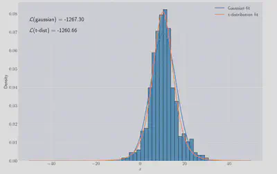
Both models visually like they fit OK but the $t$-distribution comes out with a better log-likelihood so, all else being equal, we’d pick that model to best describe out data (or better still use some kind of penalised loglikelihoodsuch as AIC and BIC!)

If we dig through the scipy documentation ⁵ we’ll find that continuous random variable like the two models we’re looking at are fitted exactly by finding the MLE values. For certain distributions, like Gaussians, we can easily derive the values of the MLE parameters so let’s do it.

For this model we have the following expression for the loglikelihood

$$\mathcal{L}(\mu ,\sigma |x_i)=\sum _i^N[\frac{1}{2}\log 2\pi {\sigma }^2-\frac{1}{2{\sigma }^2}(x_i-\mu {)}^2]$$

which we can differentiate with respect to $\mu$ and $\sigma$ to find the maxima. For $\mu$:

$$\begin{array}{r}{\partial }_{\mu }\mathcal{L}(\mu ,\sigma |x_i)=\frac{1}{{\sigma }^2}\sum _i^N(x_i-\mu )\\ \Rightarrow \sum _i^N(x_i-{\mu }_{\text{MLE}})=0\\ \Rightarrow {\mu }_{\text{MLE}}=\frac{1}{N}\sum _i^N{x}_i\equiv {\overline{x}}_i\end{array}$$

I.e. the MLE estimate for the mean parameter in a normal distribution fit is just the empirical mean. Proceeding similarly, for $\sigma$, we find:

$$\begin{array}{r}{\sigma }_{\text{MLE}}^2=\frac{1}{N}\sum _i^N(x_i-{\mu }_{\text{MLE}}{)}^2.\end{array}$$

which is the empirical standard deviation. We can confirm this is true for the dataset we have here:

print(example_data.mean(), example_data.std())
print(*n_args)
>>> 10.051125578381319 6.149058201486978
>>> 10.051125578381319 6.149058201486978

So far so good! We could do something similar for the $t$-distribution fit but the maximisation step would require a numerical method.

Gaussian Mixture Models

Things get more complicated when our model involves ’latent’ variables. Latent variables are ones for whom we never get to observe, the best we can do is to try to estimate their values. The canonical example of a latent variable model is the Gaussian Mixture Model (GMM) which we’ll go through in detail here.

Let’s build another dataset which we can then try and fit a GMM model to:

true_params = ((-5, 3), (-1, 1), (3, 1))

N, M = 999, 3

YY = [
    stats.norm(mu, sigma).rvs(N // M) for (mu, sigma) in true_params
]

and plotting that data:

_, ax = plt.subplots(figsize=(18, 7), ncols=2)

sns.histplot(YY, bins=50, ax=ax[0])

# 'Anonymise' the data
YY = np.concatenate(YY)
sns.histplot(YY, bins=50, ax=ax[1], color='b');

[a.set(xlabel=r'$x$') for a in ax];

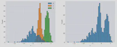
In the left-hand panel we can see the composite distributions which make up the resulting mixture, shown on the right-hand panel.

We’re going to posit that this data was generated a sum of gaussians:

$$p(x_i;{\mu }_k,{\sigma }_k)=\sum _{k=1}^K{w}_k\mathcal{N}(x_i;{\mu }_k,{\sigma }_k)$$

The problem is we don’t know

1. $K$, i.e. The true number of Gaussians we should include in our mixture
2. The parameters of these Gaussians, ${\mu }_k$ and ${\sigma }_k$
3. Which gaussian was responsible for generating each point.

The last point, (3), is really the crux of the problem since if we knew which gaussian each point was derived from then we do exactly what we did above - use a fitting procedure to calculate the mean and variance parameters and we’d be done.

This uncertainty is exactly what our latent variables encode. Let’s say we propose (correctly!) that there are three gaussians in our mixture, $K=3$, then each datapoint actually has two components: The location, $x_i$, and $z_i$ which is a one-hot vector denoting which gaussian generated the point. For example if $x_i$ was generated by the third gaussian then $z_i=(0,0,1)$.

Formally, we’re proposing that $z_i$ is drawn from a categorical distribution, parametrised by $\phi$, and that $x_i$, conditioned on $z_i=k$, is normally distributed:

$$\begin{array}{r}{x}_i|z_i=k\sim N({\mu }_k,{\sigma }_k^2),\\ z_i\sim \text{Categorical}(\phi )\end{array}$$

We can write down the likelihood for this model but because we don’t observe the $z_i$ we can’t maximise the likelihood directly, and this is where the expectation-maximisation (EM) algorithm comes in.

The EM Algorithm

Let’s derive the EM algorithm before we apply it to the GMM problem above. We start, as before, by writing down the loglikelihood over the observed data.

$$\mathcal{L}(\theta |x)=\sum _i\log p(x_i|\theta ).$$

We now need to find a way to introduce our $z_i$ somehow. A natural choice would be to substitute $p(x_i|\theta )=\sum _{z_i}p(x_i,z_i|\theta )$ but we would end up with an expression which was difficult to maximise because of the sum-inside-a-logarithm shape it would acquire. So instead we bring in the $z_i$ using the fact that $\sum _{z_i}p(z_i|x_i,{\theta }^{(n)})=1$, for some choice of ${\theta }^{(n)}$ which need not be the same as $\theta$

$$\begin{array}{rl}\mathcal{L}(\theta |x)& =\sum _i\log p(x_i|\theta )\sum _{z_i}p(z_i|x_i,{\theta }^{(n)})\\ & =\sum _i\sum _{z_i}p(z_i|x_i,{\theta }^{(n)})\log p(x_i|\theta ).\end{array}$$

The law of conditional probability allows us rewrite the term inside the logarithm as follows

$$\begin{array}{rl}\mathcal{L}({\theta }^{(n)}|x)& =\sum _i\sum _{z_i}p(z_i|x_i,{\theta }^{(n)})\log \frac{p(x_i,z_i|\theta )}{p(z_i|x_i,\theta )}\\ & =\sum _i\sum _{z_i}(p(z_i|x_i,{\theta }^{(n)})\log p(x_i,z_i|\theta )-p(z_i|x_i,{\theta }^{(n)})\log p(z_i|x_i,\theta ))\\ & =\sum _i{\mathbb{E}}_{z_i|x_i,{\theta }^{(n)}}[\log p(x_i,z_i|\theta )]-\sum _i{\mathbb{E}}_{z_i|x_i,{\theta }^{(n)}}[\log p(z_i|x_i,\theta )]\\ & ={\mathbb{E}}_{z_i|x_i,{\theta }^{(n)}}[\sum _i\log p(x_i,z_i|\theta )]-{\mathbb{E}}_{z_i|x_i,{\theta }^{(n)}}[\sum _i\log p(z_i|x_i,\theta )]\\ & ={\mathbb{E}}_{z_i|x_i,{\theta }^{(n)}}[\log \prod _{i}p(x_i,z_i|\theta )]-{\mathbb{E}}_{z_i|x_i,{\theta }^{(n)}}[\log \prod _{i}p(z_i|x_i,\theta )]\\ & \equiv \mathcal{Q}(\theta |{\theta }^{(n)})+\mathcal{H}(\theta |{\theta }^{(n)}).\end{array}$$

So, we have broken the incomplete log-likelihood into two terms:

• The ‘auxilliary’ function, $\mathcal{Q}(\theta |{\theta }^{(n)})$ – the expectation over the ‘complete data’ log-likelihood with respect to the latent variables $z_i$
• An ’entropy’ term, $\mathcal{H}(\theta |{\theta }^{(n)})$

We have all the ingredients to compute $Q$ so it would be great if we could show that maximising that was equivalent to maximising the incomplete-data log-likelihood and luckily that turns out to be the case! Starting again from the loglikelihood, but this time pursuing the sum-inside-a-logarithm approach we dodged before:

$$\begin{array}{rl}\mathcal{L}(\theta |x)& =\sum _i\log p(x_i|\theta )=\sum _i\log \sum _{z_i}p(x_i,z_i|\theta )\\ & =\sum _i\log \sum _{z_i}p(z_i|x_i,{\theta }^{(n)})\frac{p(x_i,z_i|\theta )}{p(z_i|x_i,{\theta }^{(n)})}\\ & =\sum _i\log {\mathbb{E}}_{z_i|x_i,{\theta }^{(n)}}\left[\frac{p(x_i,z_i|\theta )}{p(z_i|x_i,{\theta }^{(n)})}\right].\end{array}$$

where we have simply multiplied and divided by $p(z_i|x_i,{\theta }^{(n)})$ (again, note that ${\theta }^{(n)}$ is allowed to be different to $\theta$) and then recognised the result as an expectation.

We can now apply Jensen’s inequality for concave functions

$$\mathbb{E}[f(X)]\le f(\mathbb{E}[X])$$

to swap the expectation and the logarithm and get a lower bound on the loglikelihood:

$$\begin{array}{rl}\mathcal{L}(\theta |x)& \ge \sum _i{\mathbb{E}}_{z_i|x_i,{\theta }^{(n)}}\log \left[\frac{p(x_i,z_i|\theta )}{p(z_i|x_i,{\theta }^{(n)})}\right]\\ & =\sum _i{\mathbb{E}}_{z_i|x_i,{\theta }^{(n)}}[\log p(x_i,z_i|\theta )-\log p(z_i|x_i,{\theta }^{(n)})]\\ & =\sum _i{\mathbb{E}}_{z_i|x_i,{\theta }^{(n)}}[\log p(x_i,z_i|\theta )]-\sum _i{\mathbb{E}}_{z_i|x_i,{\theta }^{(n)}}[\log p(z_i|x_i,{\theta }^{(n)}])\\ & =\mathcal{Q}(\theta |{\theta }^{(n)})+\mathcal{H}({\theta }^{(n)}|{\theta }^{(n)})\\ \text{(*)}& \Rightarrow \mathcal{L}(\theta |x)& \ge \mathcal{Q}(\theta |{\theta }^{(n)})+\mathcal{H}({\theta }^{(n)}|{\theta }^{(n)})\end{array}$$

Now define ${\theta }^{\ast }$ as the value $\theta$ which maximises the auxilliary function, $\mathcal{Q}(\theta |{\theta }^{(n)})$, i.e.

$$\begin{array}{r}{\theta }^{\ast }={\text{argmax}}_{\theta }\mathcal{Q}(\theta |{\theta }^{(n)}),\end{array}$$

And, going step-by-step for clarity, we take $\theta ={\theta }^{\ast }$ in the equation $(\ast )$ above:

$$\begin{array}{rl}\mathcal{L}({\theta }^{\ast }|x)& \ge \mathcal{Q}({\theta }^{\ast }|{\theta }^{(n)})+\mathcal{H}({\theta }^{(n)}|{\theta }^{(n)})\end{array}$$

and by the construction of ${\theta }^{\ast }$ we have that $\mathcal{Q}({\theta }^{\ast }|{\theta }^{(n)})\ge \mathcal{Q}({\theta }^{(n)}|{\theta }^{(n)})$, therefore

$$\begin{array}{rl}\mathcal{L}({\theta }^{\ast }|x)& \ge \mathcal{Q}({\theta }^{(n)}|{\theta }^{(n)})+\mathcal{H}({\theta }^{(n)}|{\theta }^{(n)})\end{array}$$

but the right-hand side we can identify as equation $(\ast )$ again having taken $\theta ={\theta }^{(n)}$, so

$$\begin{array}{rl}\mathcal{L}({\theta }^{\ast }|x)& \ge \mathcal{L}({\theta }^{(n)}|x).\end{array}$$

which proves that maximising $Q$ is sufficient for maximising $\mathcal{L}({\theta }^{(n)}|x)$. Phew.

There is a lot going on here so lets break it down. We’ve found a function, $\mathcal{Q}(\theta |{\theta }^{(n)})$ which, for all values of $\theta$, is a lower bound to the log-likelihood $\mathcal{L}({\theta }^{(n)}|x)$. This means that we can pick an arbitrary value for $\theta$ and maximise $\mathcal{Q}$ to find the value ${\theta }^{\ast }$, then iterate.

The schematic figure below illustrates this process. We start with some guess ${\theta }_0$, find the value for $\theta$ which maximises $\mathcal{Q}(\theta |{\theta }_0)$, set that as ${\theta }_1$ and repeat.

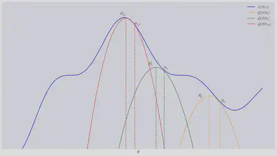
In summary, the EM algorithm breaks down into two steps:

1. E-step: Given values for ${\theta }_i$, compute $\mathcal{Q}(\theta |{\theta }_i)$,
2. M-step: Maximise $\mathcal{Q}(\theta |{\theta }_i)$ to get ${\theta }_{i+1}$.

We repeat these steps until we’re happy it has converged (using either the log-likelihood of convergence of the parameters, $\theta$, to stable values).

Fitting Gaussian Mixture Models using EM

Let’s apply all this to the Gaussian Mixture Model. As a reminder, the full model is:

$$\begin{array}{r}{x}_i|z_i=k\sim N({\mu }_k,{\sigma }_k^2),\\ z_i\sim \text{Categorical}(\phi )\end{array}$$

where $0\le {\phi }_k\le 1$ and $\sum _k{\phi }_k=1$.

The E-step demands that we compute the auxilliary function:

$$\begin{array}{rl}\mathcal{Q}(\theta |{\theta }^{(n)})& =\sum _i{\mathbb{E}}_{z_i|x_i,{\theta }^{(n)}}[\log p(x_i,z_i|\theta )],\\ & =\sum _i{\mathbb{E}}_{z_i|x_i,{\theta }^{(n)}}[\log \prod _k({\phi }_{k}p(x_i|{\theta }_k){)}^{\text{I}(z_i=k)}],\\ & =\sum _i{\mathbb{E}}_{z_i|x_i,{\theta }^{(n)}}[\sum _k\text{I}(z_i=k)\log ({\phi }_{k}p(x_i|{\theta }_k))].\end{array}$$

where we have writen the categorical distribution as a product using an indicator variable.

The term in the log is constant with respect to the expectation so we need only the expectation of the indicator which is given by

$$\sum _{z_i}p(z_i|x_i,{\theta }^{(n)})\text{I}(z_i=k)=p(z_i=k|x_i,{\theta }^{(n)})$$

therefore

$$\mathcal{Q}(\theta |{\theta }^{(n)})=\sum _i\sum _{k}p(z_i=k|x_i,{\theta }^{(n)})\log ({\phi }_{k}p(x_i|{\theta }_k)).$$

We can calculate the posterior over the $z$’s fairly easily, and for neatness let $w_{ik}=p(z_i=k|x_i,{\theta }^{(n)})$ in what follows

$$\begin{array}{rl}{w}_{ik}& =\frac{p(x_i,z_i=k|{\theta }^{(n)})}{p(x_i|{\theta }^{(n)})}=\frac{p(x_i,z_i=k|{\theta }^{(n)})}{\sum _{z_i}p(x_i,z_i|{\theta }^{(n)})},\\ & =\frac{{\phi }_k\mathcal{N}(x_i|{\mu }_k,{\sigma }_k^2)}{\sum _j{\phi }_j\mathcal{N}(x_i|{\mu }_j,{\sigma }_j^2)}.\end{array}$$

Therefore,

$$\mathcal{Q}(\theta |{\theta }^{(n)})=\sum _i\sum _k{w}_{ik}(\log {\phi }_k^{(n)}+\log \mathcal{N}(x_i|{\mu }_k^{(n)},{\sigma }_k^{2(n)}))).$$

That’s the E-step done. The M-step requires us maximise this expression to get an update rule for the model parameters. I’ll demonstrate this is only for ${\phi }_k$ because it follows similarly for the other parameters. It is a constrained optimisation problem because of the contrain on the ${\phi }_k$’s, therefore we need to use Lagrange multipliers:

$$\begin{array}{rl}L& =\sum _i\sum _k{w}_{ik}\log {\phi }_k+\alpha (\sum _k{\phi }_k-1)\\ \frac{\partial L}{\partial {\phi }_j}& =\sum _i\frac{w_{ij}}{{\phi }_j}+\alpha =0\end{array}$$

and the constraint over $\phi$ gives

$${\phi }_k^{(n+1)}=\frac{1}{N}\sum _i{w}_{ik}.$$

The other update rules are:

$$\begin{array}{rl}{\mu }_k^{(n+1)}& =\frac{\sum _i{w}_{ik}{x}_i}{\sum _i{w}_{ik}}\\ {\sigma }_k^{2(n+1)}& =\frac{\sum _i{w}_{ik}(x_i-{\mu }_k^{(n)}{)}^2}{\sum _i{w}_{ik}}\end{array}$$

and that condlues the M-step. We can now implement this and see if we can fit the dataset.

Implementing EM for GMMs in python

from typing import Tuple


def get_initial_guess_for_mus(YY: np.array, n_components: int) -> np.array:
    # Choose some sensible percentiles
    return np.percentile(YY, np.linspace(0, 100, n_components + 2)[1: -1])


def compute_q(w_ik, phis, mus, sigmas, YY):
    N, n_components = w_ik.shape
    return np.sum([
        w_ik[i, k] * (np.log(phis[k]) + stats.norm(mus[k], np.sqrt(sigmas[k])).logpdf(YY[i]))
        for i in range(N)
        for k in range(n_components)
    ])


def compute_h(w_ik):
    N, n_components = w_ik.shape
    return - np.sum([
        w_ik[i, k] * np.log(w_ik[i, k])
        for i in range(N)
        for k in range(n_components)
    ])



def fit_gmm_with_em(YY: np.array, n_components: int, em_itrs: int=10) -> Tuple[np.array]:
    N = YY.shape[0]

    phis = np.ones(n_components) / n_components
    range_ = YY.max() - YY.min()
    sigmas = np.ones(n_components)
    w_ik = np.zeros((N, n_components))
    mus = get_initial_guess_for_mus(YY, n_components)

    for itr in range(em_itrs):
        # E-step
        w_ik = np.array([
            phis[k] * stats.norm(mus[k], np.sqrt(sigmas[k])).pdf(YY[i])
            for i in range(N)
            for k in range(n_components)
        ]).reshape(N, n_components)
        w_ik = w_ik / w_ik.sum(axis=1)[:, np.newaxis]

        # M-step
        sum_i_w_ik = w_ik.sum(axis=0)
        phis = sum_i_w_ik / N
        mus = (w_ik.T.dot(YY)) / sum_i_w_ik
        sigmas = w_ik.T.dot((YY[:, np.newaxis] - mus) ** 2).diagonal() / sum_i_w_ik

        # Compute the value of the Q function at our current parameters
        print(itr, compute_q(w_ik, phis, mus, sigmas, YY))

    return w_ik, phis, mus, sigmas

w_ik, phis, mus, sigmas = fit_gmm_with_em(YY, 3)

We can plot the individual gaussians as well as the resulting mixture to check the fit:

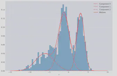
It looks like a much better fit than if we’d used a single gaussian! We can also calculate the log-likelihood of the GMM fit, to what we can achieve if we just fit a single Gaussian to the data:

# Our proxy objective function, Q
Q = compute_q(w_ik, phis, mus, sigmas, YY)

# The entropy term, H
H = compute_h(w_ik)

single_gaussian_ll = calculate_ll(stats.norm, n_args, xx)

print(Q + H, single_gaussian_ll)
>>> -2586.743170746824, -2748.671049075651

Unsuprisingly the mixture model gives a much better fit!

Closing Remarks

We’ve derived and then applied the Expectation-Maximisation algorithm to some simple fake one-dimensional data and shown that it outperformed the naive single gaussian fit by checking the log-likelihood of the two approaches.

In part 2 of this blog I’ll take the theory explained here and look at a very different application: How we can deal with ‘censored data’ problems (where data is, for whatever reason, only partially observed) using expectation maximisation.

References