Online Bayesian Learning Part 1: Exact recursive inference

Preamble

This is the first of a three post series in which I’ll explore a few ideas I recently came across while reading Gerardo Martin’s thesis [1] and more recently also in the book Bayesian Filtering And Smoothing [2]. The introductory chapters of which I’ll be following closely in these posts. The topics in [1] relate to the challenges which arise in ‘sequential machine learning’: Models where we do not have a complete dataset to train on, before deploying it in some (hopefully stationary) setting. Instead we get to observe data as they arrive through time, and can update our beliefs about the underlying model accordingly. Although this sort of ‘streaming’ data is all too common, in my experience it is often handled by constructing models on a fixed snapshot of past data, deploying, and then periodically retraining when enough new data has arrived or a model’s predictive power is suspected of being in decline. The recursive approach we’ll explore is particularly useful in scenarios with memory constraints, real-time requirements, or when data arrives continuously and storing all historical observations is impractical.

In this post I’ll start out by implementing a simple Bayesian ridge regression for sequential data. Everything here will be exact but will serve as a spring board for trickier problems to come as well as an introduction to building Bayesian neural networks (BNNs).

In the second post I’ll extend this to non-linear measurement models which will not have closed-form expressions. Instead we will use variational inference to approximate the true distributions of our model parameters in order for us to describe these data.

Finally in the third post we’ll see how these ideas can be intuitively extended so that non-stationary streaming data can be well modelled.

All code in these posts will be implemented using JAX [3]. I’ll also use Equinox [4], a JAX-based neural network library that provides a neat, PyTree-compatible approach to building and training neural networks.

A jupyter notebook version of the code in this post is available here.

Bayesian Neural Networks: Introduction

Here I am predominantly interested in the application of BNNs because they apply naturally to tasks where we are afforded the opportunity to update our beliefs through time, but it is worth mentioning the other main advantage that they bring: Parameter uncertainty, and therefore prediction uncertainty.

Standard neural networks are constructed from weights and biases which are single floating point values, they learn the single best values for the model parameters that minimise our loss function (or at least the parameters which locate for us a local optima). While this approach works well for many applications, it fundamentally ignores the uncertainty inherent in learning with finite resources, both finite data and finite compute. When a neural network predicts that…

• a house is worth £500k
• an image of a tumour shows a growth which is benign
• it is perfectly safe for a self-driving car to turn left across two lanes of busy traffic in San Francisco (as I experienced personally…)

how confident should we be in that prediction? Are our models equally uncertain about all predictions, or are some regions of input space more reliable than others? Given a regression problem where we have lots of training data in some regions of but sparse data elsewhere a standard neural network will make confident predictions everywhere, even in regions where it has never seen data.

There are ways to coax a non-Bayesian network into giving a range of predictions (and therefore a sort of estimate of uncertainty): We can use inference-time dropout, or we can build ensembles of models each trained on subsets. In contrast BNNs offer a principled framework for quantifying this uncertainty by treating network weights as random variables rather than fixed parameters.

It is, however, worth pointing out that BNNs are not a panacea. They are harder and slower to train so we find ourselves restricted to less fancy architectures, with fewer parameters. It is also clear from the success of LLMs in the past few years that sometimes a point estimate is ‘good enough’!

Bayesian Neural Networks: Theory

In the Bayesian framework, we place a prior distribution over network weights and use Bayes’ theorem to compute the posterior distribution given observed data:

$$p(\theta | \mathcal{D}) = \frac{p(\mathcal{D} | \theta) p(\theta)}{p(\mathcal{D})}$$

Where $\theta$ represents all of our network parameters, $\mathcal{D} = {(x_i, y_i)}_{i=1}^N$ is our training data. $p(\theta)$ is our prior for the network parameters, $p(\mathcal{D} | \theta)$ is the likelihood, and $p(\mathcal{D})$ is the marginal likelihood or evidence. The posterior, $p(\theta | \mathcal{D})$, encodes our updated beliefs about the parameters after observing the data, $\mathcal{D}$.

To make predictions on new inputs $x^*$, we integrate over this posterior:

$$p(y^{*} | x^{*}, \mathcal{D}) = \int p(y^{*} | x^{*}, \theta) p(\theta | \mathcal{D}) d\theta$$

The shape of this posterior predictive distribution quantifies our uncertainty: confident predictions are represented by low distributional variance, and uncertain predictions with high variance.

The challenge usually lies in computing the posterior $p(\theta | \mathcal{D})$. For neural networks with a large number of parameters the normalizing constant $p(\mathcal{D})$ requires integrating over an extremely high-dimensional space, making exact inference intractable. In the second and third posts in this mini-series we will use approximate inference methods to compute our posteriors but for now let’s look at an example which admits an exact solution.

Recursive Ridge Regression

As ever, it begins with linear regression! Specifically a multi-dimensional Bayesian linear regression where we assume Gaussian priors for our parameters and assume a Gaussian likelihood:

$$\begin{align*} p(\theta) &= \mathcal{N}(\mu_0, \Sigma_0), \\ p(y_t | X_t, \theta) &= \mathcal{N}(X_t \theta, \sigma^2 I), \end{align*}$$

where $\theta \in \mathbb{R}^k$ is the parameter vector, $X_t \in \mathbb{R}^{n \times k}$ contains $n$ observations of the $k$-dimensional features at time $t$, $\sigma$ is assumed known and constant and observations are assumed to have uncorrelated noise terms.

As stated above our dataset will be ‘streamed’ to us and this is the role that the $t=0, 1, \ldots, T$ index is playing. In this post, and the subsequent follow ups, new data will arrive in batches of a constant size at each new time step. Technically then, the data are indexed ${(x_{t,i}, y_{t,i})}_{t=1,i=1}^{T, N}$ but this is a bit messy so I will suppress the $i$ index unless it is required.

We can derive the update equations from first principles. We start with a Gaussian prior over parameters and a new batch of data $(X_t, y_t)$ with Gaussian likelihood:

By Bayes’ rule, the posterior is:

$$p(\theta_t | X_t, y_t) \propto p(y_t | X_t, \theta_t) p(\theta_{t-1} | \mathcal{D}_{t-1})$$

Since both our prior and likelihood are Gaussian, the posterior is also Gaussian [4]. To see this, we start with the log of the unnormalized posterior:

$$\begin{align*} \log p(\theta_t | X_t, y_t) &\propto \log p(y_t | X_t, \theta_t) + \log p(\theta_t) \\ &= -\frac{1}{2\sigma^2}(y_t - X_t\theta_t)^T(y_t - X_t\theta_t) - \frac{1}{2}(\theta_t - \mu_{t-1})^T\Sigma_{t-1}^{-1}(\theta_t - \mu_{t-1}) \end{align*}$$

Expanding the quadratic terms and collecting terms in $\theta_t$:

$$\begin{align*} \log p(\theta_t | X_t, y_t) &\propto -\frac{1}{2}\theta_t^T\left(\Sigma_{t-1}^{-1} + \frac{X_t^TX_t}{\sigma^2}\right)\theta_t \\ &\quad+\theta_t^T\left(\Sigma_{t-1}^{-1}\mu_{t-1} + \frac{X_t^Ty_t}{\sigma^2}\right) + \text{const} \end{align*}$$

Comparing with the standard Gaussian form $-\frac{1}{2}\theta_i^T\Sigma^{-1}\theta_i + \theta_i^T\Sigma^{-1}\mu$, we identify that the posterior covariance is given by:

$$\Sigma_t^{-1} = \Sigma_{t-1}^{-1} + \frac{X_t^TX_t}{\sigma^2}$$

and similarly

$$\mu_t = \Sigma_t\left(\Sigma_{t-1}^{-1}\mu_{t-1} + \frac{X_t^Ty_t}{\sigma^2}\right).$$

The mean update rule requires $\Sigma_t$ directly. We can get this with an application of the Sherman-Morrison-Woodbury formula (SMW) [5]. SMW states that for matrices $A\in\mathbb{R}^{n\times n}, C\in\mathbb{R}^{k\times k}, U\in\mathbb{R}^{n\times k}, V\in\mathbb{R}^{k\times n}$:

$$(A + UCV)^{-1} = A^{-1} - A^{-1}U(C^{-1} + VA^{-1}U)^{-1}VA^{-1}.$$

We take $A = \Sigma_{t-1}^{-1}$, $U = X_t^T$, $C = \frac{1}{\sigma^2}I$ and $V = X_t$ to yield our result for the posterior covariance:

$$\begin{align*} \Sigma_t &= \left(\Sigma_{t-1}^{-1} + \frac{X_t^TX_t}{\sigma^2}\right)^{-1} \\ &= \Sigma_{t-1} - \Sigma_{t-1} X_t^T(\sigma^2 I + X_t\Sigma_{t-1} X_t^T)^{-1} X_t \Sigma_{t-1}. \end{align*}$$

The recursive updates are mathematically equivalent to computing the full batch posterior $p(\theta|X_{1:t}, y_{1:t})$ at each time step, where the batch solution requires inverting the full accumulated information matrix:

$$\Sigma_t = \left(\Sigma_0^{-1} + \frac{1}{\sigma^2}\sum_{i=1}^t X_i^T X_i\right)^{-1}$$

This batch approach becomes computationally prohibitive as the size of the dataset grows, since we must invert an increasingly large sum of matrices at each step, whereas the recursive formulation maintains constant computational complexity per update.

And with that, we have all we need to implement our model. But first, a short aside…

The Kalman Filter

The recursive structure we’ve derived is actually equivalent to the well known Kalman filter. If we define the Kalman gain $K_t = \Sigma_{t-1} X_t^T(\sigma^2 I + X_t\Sigma_{t-1} X_t^T)^{-1}$, our updates can be rewritten as:

$$\begin{align*} \mu_t &= \mu_{t-1} + K_t(y_t - X_t\mu_{t-1}) \\ \Sigma_t &= \Sigma_{t-1} - K_t X_t \Sigma_{t-1} \end{align*}$$

This form makes the intuition clearer: we correct our prior mean $\mu_{t-1}$ by the prediction error $(y_t - X_t\mu_{t-1})$, weighted by our confidence in that prediction through $K_t$. While the covariance shrinks as we gain information, with the reduction proportional to how informative the new data is.

Implementation

Before we build the model itself, we must build a little dataset for us to train on. We will take $k=4$ features, two of which are related to our response, $y$, and two of which are just adding noise.

 1
 2
 3
 4
 5
 6
 7
 8
 9
10
11
12
13
14
15
16
17

def generate_data_stream(key, theta, *, T, n, std):
    n_parameters = theta.shape[0]
    XX, yy = [], []
    for _ in range(T):
        key, k1, k2 = jax.random.split(key, 3)
        X_t = jax.random.normal(k1, (n, n_parameters))
        noise = std * jax.random.normal(k2, (n,))
        y_t = X_t @ theta + noise
        XX.append(X_t)
        yy.append(y_t)
    return jnp.array(XX), jnp.array(yy)


# One positively correlated, one negatively correlated, and two uncorrelated:
true_theta = jnp.array([1.0, -1.5] + [0.0] * 2)
key = jax.random.PRNGKey(0)
XX, yy = generate_data_stream(key, true_theta, T=50, n=5, std=0.5)

We can visualise this, sampling a handful of the times:

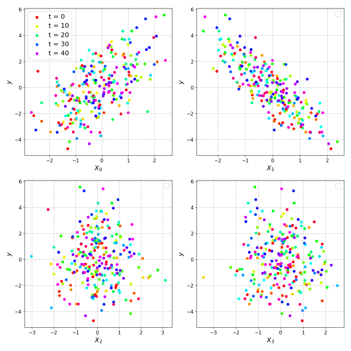
The correlation is clear for $X_0$ and $X_1$ when we are able to see a large number of data points (i.e. all of the shades of colour), but there is a fair amount of noise in the relationship.

To update our posterior beliefs at each time step: we use the recursive_ridge_update function defined here:

 1
 2
 3
 4
 5
 6
 7
 8
 9
10
11
12
13
14
15
16
17
18
19
20
21
22
23
24
25
26

class GaussianPosterior(NamedTuple):
    mean: jnp.ndarray
    covariance: jnp.ndarray


def recursive_ridge_update(
    previous_posterior: GaussianPosterior,
    X: jnp.ndarray,
    y: jnp.ndarray,
    sigma2: float,
) -> GaussianPosterior:
    # To be explicit: the posterior at (t-1) becomes the prior at t
    prior = previous_posterior

    # Compute intermediate matrices
    n, _ = X.shape
    S_t = sigma2 * jnp.eye(n) + X @ prior.covariance @ X.T
    K_t = prior.covariance @ X.T @ jnp.linalg.inv(S_t)

    # Posterior mean update:
    mu_t = prior.mean + K_t @ (y - X @ prior.mean)

    # Posterior covariance update:  
    sigma_t = prior.covariance - K_t @ X @ prior.covariance

    return GaussianPosterior(mean=mu_t, covariance=sigma_t)

and then we simply iterate over our data batches, updating as we go:

 1
 2
 3
 4
 5
 6
 7
 8
 9
10
11
12
13
14
15
16
17
18
19
20
21

def fit_recursive_ridge(
    XX: jax.Array,
    yy: jax.Array,
    sigma2: float = 1.0,
    prior_variance: float = 2.0,
):
    _, n_features = XX[0].shape
    posterior = GaussianPosterior(
        mean=jnp.zeros(n_features), 
        covariance=prior_variance * jnp.eye(n_features)
    )

    posteriors = []
    for X_t, y_t in zip(XX, yy):
        posterior = recursive_ridge_update(posterior, X_t, y_t, sigma2)
        posteriors.append(posterior)

    return posteriors


posteriors = fit_recursive_ridge(XX, yy)

Results and Analysis

Plotting the posterior means for each coefficient, along with their $\pm2\sigma$ uncertainty regions through time:

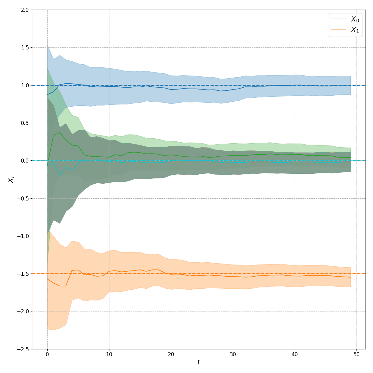
we can see that even after a few time steps our model’s coefficient posteriors nicely capture the true values, while the coefficients which were uncorrelated to the response have collapsed quickly towards zero. The coefficient posterior variance shrinks over time but doesn’t collapse rapidly to zero. Since the features $X_t$ are drawn from a standard normal distribution, the eigenvalues of the information matrices $X_t^T X_t$ remain bounded, limiting how much the posterior precision $\Sigma_t^{-1}$ can grow with each update. This bounded information gain per time step, combined with the observation noise $\sigma^2$, leads to gradual rather than rapid uncertainty reduction.

Next Steps

In this example we were able to derive analytic closed-form for the posterior in the case of a linear measurement model. In the next post, we’ll introduce the Recursive Variational Gaussian Approximation (R-VGA) [6] which enables efficient online learning for non-linear measurement models (i.e. neural networks) in streaming data scenarios.

References

[1]: Adaptive, Robust and Scalable Bayesian Filtering for Online Learning - Gerardo Duran-Martin

[2]: Bayesian Filtering And Smoothing - Simo Särkkä

[3]: JAX: Composable transformations of Python+NumPy programs

[4]: Equinox: Elegant easy-to-use neural networks + scientific computing in JAX

[5]: Woodbury matrix identity - Wikipedia

[6]: The recursive variational Gaussian approximation (R-VGA) - Marc Lambert, Silvere Bonnabel, Francis Bach