Online Bayesian Learning Part 2: Bayesian Neural Networks With Variational Inference

Introduction

In Part 1, we implemented Bayesian inference for linear regression using conjugate Gaussian priors and likelihoods. In this simple model the recursive updates resulted in exact posterior distributions that we could update efficiently as new data arrived.

The eventual goal of this mini-series is to understand and implement the Recursive Variational Gaussian Approximation (R-VGA) but to get there we first need a brief introduction to Variational Inference (VI) [1]. VI has been written about extensively, and by people better versed in it than I am [2]. But it’s an important stepping stone to R-VGA and the machinery developed here will be useful later on so including a quick introduction to VI here seems a worthwhile inclusion.

In this post we’ll train a small non-Bayesian neural network (NN) to perform a regression task on some fake data. We will then swap this for a Bayesian Neural Net (BNN) with the same architecture (indeed, the same model code!) and see how we can use VI to train this. As in the rest of this series all models will be constructed using JAX and equinox.

A jupyter notebook version of the code in this post is available here.

Bayesian neural networks

NNs are composed of ’layers’ of linear transformations and non-linear ‘activations’. The linear transformations are usually matrix products but can be fancier constructs like convolutions [3] or attention blocks [4]. The activations range from simple analytic functions like the ReLU, GELU or sigmoid function, but more involved non-linearities are also possible. For example, the SwiGLU function is a non-linearity which has its own learnable parameters.

Part 1 introduced and implemented a model which can be viewed as the simplest possible neural network: we got our model prediction by taking a single linear transformation (a dot product) of the model weights (the regression coefficients, $\theta$) and the model inputs (the features, $X$).

There, we found that our Bayesian update rules were pleasingly simple and even better, they yielded exact expressions. So can we expect that the same will be the case for more general BNNs? Unfortunately not…There are a few reasons why things are more complicated for non-trivial neural network architectures:

Conjugacy: In part 1, the fact that our posterior ended up being from the same family as our prior was a result of ‘conjugacy’. There are lots of other examples of conjugate models [5], but in general neural networks with their non-linearities are not among them. This means that if we really want our posterior distribution, we will be faced with some tricky integrals to evaluate.
Dimensionality: NNs are typically massively over-parametrised: it’s not unusual for a model to contain tens if not hundreds of thousands of model weights. This means that the integrals mentioned just above are not only going to need some sort of approximations to compute, they are going to be massively multi-dimensional and our favourite tricks for approximating integrals do not scale nicely with dimension.
The evidence term: The $p(\mathcal{D})$ in Bayes’ formula which we wrote down to compute the posterior before is also difficult. In part 1 we were able to skip over this by simply identifying the form of our updates but not any more!

It is worth pointing out that despite these issues it is still possible to perform exact inference for these models. We can use Markov Chain Monte Carlo (MCMC) to build our posteriors, see [6] for a great run through of this using the python package pymc [7]. Granted, these are only exact in the limit where we can draw an infinite number of MCMC samples and pymc’s own documentation impresses that VI, which it also implements, as being preferable to sampling when scaling models to large datasets.

Variational Inference

When applying variational inference techniques, we give up on computing the true posterior over the parameters of our BNN, $p(\theta|\mathcal{D})$, and instead aim to find the best approximation for it, $q(\theta)\in\mathcal{Q}$ where $\mathcal{Q}$ is our family of approximating densities. Typically we take $\mathcal{Q}$ to be ’the family of all normal distributions’ i.e. $\mathcal{Q} = \{\mathcal{N}(\mu, \Sigma)\}$.

Rather than sampling from cleverly constructed Markov chains we aim to find the distribution $q(\theta)\in\mathcal{Q}$ which is closest to the true posterior, where the definition of “closest” is defined by as that which minimises the KL divergence between the target distribution and the approximating distribution. As a reminder, the KL divergence between a distribution $p(x)$ and $q(x)$ is defined as

$$ D_{\text{KL}}(q || p) = \mathbb{E}_{x\sim q(x)}\left[\log\frac{q(x)}{p(x)}\right]. $$

The distribution in $\mathcal{Q}$ which closest approximates the true posterior is therefore given by

$$ \begin{align*} q^*(\theta) &= \argmin_{q\in\mathcal{Q}} D_{\text{KL}}(q(\theta) || p(\theta|\mathcal{D})) \\ &= \argmin_{q\in\mathcal{Q}} D_{\text{KL}}\left(q(\theta) || \frac{p(\mathcal{D}|\theta)p(\theta)}{p(\mathcal{D})}\right) \end{align*} $$

We note that the KL divergence involves the troublesome evidence term $p(\mathcal{D})$ which we were trying to avoid in the first place. Fortunately, we can derive a tractable objective which is provably equivalent to this. Starting from the definition of the KL divergence:

$$ \begin{align*} D_{\text{KL}}(q(\theta) || p(\theta|\mathcal{D})) &= \mathbb{E}_{\theta\sim q}[\log q(\theta)] - \mathbb{E}_{\theta\sim q}[\log p(\theta | \mathcal{D})] \\ &= \mathbb{E}_{\theta\sim q}[\log q(\theta)] - \mathbb{E}_{\theta\sim q}[\log p(\theta, \mathcal{D})] + \mathbb{E}_{\theta\sim q}[\log p(\mathcal{D})] \end{align*} $$

where we have simply started with the definition of the KL divergence and then expanded the conditional. But $p(\mathcal{D}$) has no $\theta$ dependence so the last expectation can be dropped:

$$ \begin{align*} D_{\text{KL}}(q(\theta) || p(\theta|\mathcal{D})) &= \mathbb{E}_{\theta\sim q}[\log q(\theta)] - \mathbb{E}_{\theta\sim q}[\log p(\theta, \mathcal{D})] + \log p(\mathcal{D}) \end{align*} $$

or another way:

$$ \begin{align*} \log p(\mathcal{D}) = D_{\text{KL}}(q(\theta) || p(\theta|\mathcal{D})) - \mathbb{E}_{\theta\sim q}[\log q(\theta)] + \mathbb{E}_{\theta\sim q}[\log p(\theta, \mathcal{D})] \end{align*} $$

Since $\log p(\mathcal{D})$ is a constant with respect to our variational distribution, $q(\theta)$, minimising the target KL divergence term is equivalent to maximising the ‘Evidence Lower Bound’ (ELBO):

$$ \text{ELBO} = \mathbb{E}_{\theta\sim q}[\log p(\theta, \mathcal{D})] - \mathbb{E}_{\theta\sim q}[\log q(\theta)]. $$

Rewriting the $p(\theta, \mathcal{D})$ term as a conditional distribution

$$ \begin{align*} \text{ELBO} &= \mathbb{E}_{\theta\sim q}[\log p(\theta)] + \mathbb{E}_{\theta\sim q}[\log p(\mathcal{D}|\theta)] - \mathbb{E}_{\theta\sim q}[\log q(\theta)] \\ &= \mathbb{E}_{\theta\sim q}[\log p(\mathcal{D}|\theta)] - D_{\text{KL}}(q(\theta) || p(\theta)) \end{align*} $$

we can see that the ELBO decomposes neatly into two intuitive terms:

Likelihood term: $\mathbb{E}_{q(\theta)}[\log p(\mathcal{D}|\theta)]$ measures how well parameters sampled from $q(\theta)$ fit the data
KL regularization term: $D_{\text{KL}}(q(\theta) || p(\theta))$ penalizes deviations from the prior

To make optimization computationally feasible, we typically assume that the parameters are independent and therefore our VI distribution factorises conveniently:

$$ q(\theta) = \prod_{i=1}^{P} q(\theta_i) $$

where $P$ is the total number of parameters in our neural network. This ‘mean field’ assumption ignores correlations between parameters but makes the optimization tractable. For neural networks with thousands of even millions of parameters, computing the full covariance matrix would be computationally infeasible.

In this model (and indeed in every application of VI I’ve seen) we choose our $\mathcal{Q}$ family to be the Gaussian distributions, i.e.

$$ q(\theta_i) = \mathcal{N}(\theta_i| \mu_i, \sigma_i^2) $$

Our variational parameters are therefore ${\mu_i, \sigma_i}$ for each network weight, and we end up with double the number of parameters in our model than in the non-Bayesian case.

With these choices made, our KL divergence takes the following form:

$$ \text{KL}\left(q(\theta)|p(\theta)\right) = \frac12 \sum_{i=1}^k \left( \frac{\sigma_i^2+\mu_i^2}{\sigma_p^2} - 1 - 2\log\frac{\sigma_i}{\sigma_p} \right) $$

When optimising the ELBO using stochastic gradient descent we have to compute gradients ’through’ the expectation $\mathbb{E}_{q(\theta)}[\log p(\mathcal{D}|\theta)]$. Since this involves sampling from $q(\theta)$, naive approaches (for example, REINFORCE: where we estimate the gradient using a small number of Monte Carlo samples) would result in high-variance gradient estimates. A better approach is found in the ‘reparameterization trick’ [8] which solves this by rewriting the sampling process trivially as:

$$ \theta_i = \mu_i + \sigma_i \epsilon_i $$

where $\epsilon_i \sim \mathcal{N}(0, 1)$. Now the randomness is isolated in $\epsilon_i$, while the $\mu_i$ and $\sigma_i$ parameters of our neural network can be updated using normal backpropagation rules.

Implementation

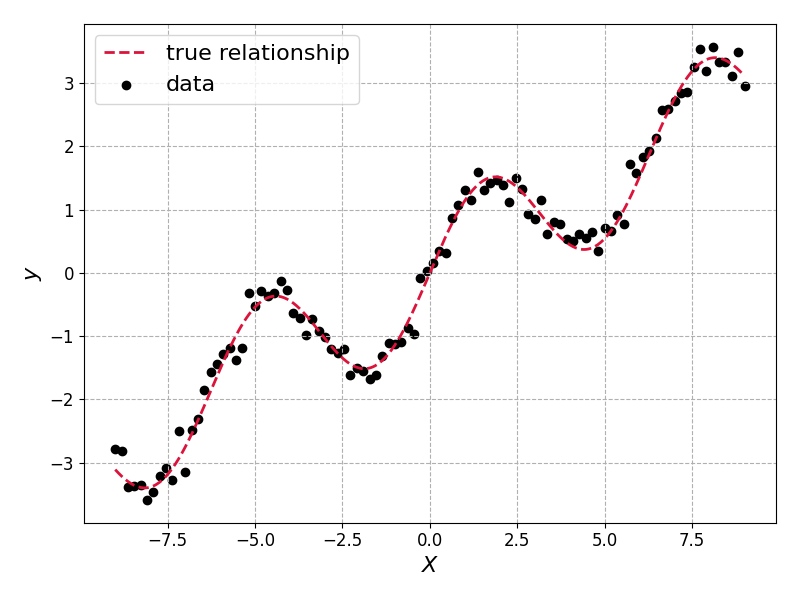
Now to the implementation. We’ll train a Bayesian neural network using variational inference and compare it with a standard (non-Bayesian) network. We’ll use a 1D regression task with a toy dataset.

 1
 2
 3
 4
 5
 6
 7
 8
 9
10
11
12
13
14
15
16
17
import jax
import jax.numpy as jnp
import equinox as eqx
import optax
from functools import partial
from typing import NamedTuple
from jax.flatten_util import ravel_pytree

key = jax.random.PRNGKey(0)
n = 100
x = jnp.linspace(-9, 9, n).reshape(-1, 1)

def true_fn(x):
    return jnp.sin(x) + 0.3 * x

obs_noise = 0.2
y = true_fn(x) + obs_noise * jax.random.normal(key, shape=x.shape)

The true relationship, true_fn, and the sampled data $\{X_i, y_i\}$ look like this:

VI toy training data

The model we’ll learn in both cases is a simple two layer MLP. We will use this for the Bayesian and non-Bayesian models:

 1
 2
 3
 4
 5
 6
 7
 8
 9
10
11
12
13
14
15
16
17
class MLP(eqx.Module):
    layers: list

    def __init__(self, key):
        keys = jax.random.split(key, 3)
        self.layers = [
            eqx.nn.Linear(1, 16, key=keys[0]),
            jax.nn.tanh,
            eqx.nn.Linear(16, 16, key=keys[1]),
            jax.nn.tanh,
            eqx.nn.Linear(16, 1, key=keys[2]),
        ]

    def __call__(self, x):
        for layer in self.layers:
            x = layer(x)
        return x

The non-Bayesian model

We can now train this optimising the MSE loss, using the optax optimisation package to handle our gradient updates for us.

<skippable details specific to jax>

Click to expand

This part is skippable for those who don’t want to worry about the finer points of the implementation, or are already familiar with jax:

The manual partitioning and flattening steps below are specifically needed for variational inference, not for basic neural network training. For VI, we need:

Flat parameter vectors: To create VariationalParams with matching shapes for mean and log_std
Easy sampling: The reparameterization trick works cleanly with flattened arrays
Optimizer compatibility: optax optimizers expect flat parameter vectors

We split the model into:

Arrays (weights/biases): The parameters we’ll make variational
Static parts (activation functions): Fixed model structure

The model_unflatten function reconstructs the full model from flattened parameters. Note that for standard (non-Bayesian) training, you could skip all this partitioning and use equinox’s eqx.filter_value_and_grad and eqx.apply_updates directly on the model.

On to the code…

</skippable details specific to jax>

First we build the loss, initialise the model and flatten its parameters:

 1
 2
 3
 4
 5
 6
 7
 8
 9
10
11
12
13
14
15
16
def mse_loss(params, model_unflatten, x, y):
    model = model_unflatten(params)
    preds = jax.vmap(model)(x)
    return jnp.mean((preds - y) ** 2)

key, subkey = jax.random.split(key)
standard_model = MLP(subkey)

model_arrays, model_static = eqx.partition(standard_model, eqx.is_array)
flat_params, unravel_arrays = ravel_pytree(model_arrays)

def unflatten(static, flat_params):
    arrays = unravel_arrays(flat_params)
    return eqx.combine(arrays, static)

model_unflatten = partial(unflatten, model_static)

and then we build a little training loop:

 1
 2
 3
 4
 5
 6
 7
 8
 9
10
11
12
13
14
15
16
17
optimizer = optax.adam(1e-2)
opt_state = optimizer.init(flat_params)

@eqx.filter_jit
def step(params, model_unflatten, opt_state, x, y):
    def loss_fn(params_):
        return mse_loss(params_, model_unflatten, x, y)
    
    loss_val, grads = jax.value_and_grad(loss_fn)(params)
    updates, opt_state = optimizer.update(grads, opt_state)
    params = optax.apply_updates(params, updates)
    return params, opt_state, loss_val

for _ in range(1000):
    flat_params, opt_state, loss = step(
        flat_params, model_unflatten, opt_state, x, y
    )

A quick check of the model loss as we moved through the epochs, and the predictions which we get from the model:

Standard MLP training loss

Standard MLP predictions

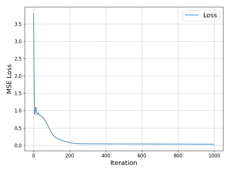
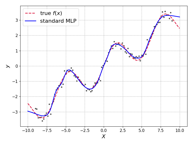
It fits well. Arguably too well as it has overfit in some places but we needn’t worry too much for this toy dataset.

Our non-Bayesian model gives us only a single prediction, with no measure of uncertainty available.

The Bayesian model

Now we implement the Bayesian version using variational inference. First, we define a little structure to hold our variational parameters:

1
2
3
class VariationalParams(NamedTuple):
    mean: jnp.ndarray
    log_std: jnp.ndarray

Standard deviations must be positive, so to keep our optimisation procedure unconstrained we store the log-standard deviations.

The reparameterization trick, in code, is simply the following

1
2
3
def sample_params(params: VariationalParams, key: jax.Array) -> jnp.ndarray:
    eps = jax.random.normal(key, params.mean.shape)
    return params.mean + jnp.exp(params.log_std) * eps

Our ELBO implementation combines the likelihood and KL divergence terms as derived above

 1
 2
 3
 4
 5
 6
 7
 8
 9
10
11
12
13
14
15
16
17
18
19
20
21
22
23
24
25
def elbo(
    params: VariationalParams,
    x: jnp.ndarray,
    y: jnp.ndarray, 
    unflatten,
    key: jax.Array,
) -> float:
    # Sample model parameters using reparameterization trick
    sample = sample_params(params, key)
    model = unflatten(sample)

    # log-likelihood calculation:
    batch_preds = jax.vmap(model)(x)
    ll = -0.5 / obs_noise**2 * jnp.sum((batch_preds - y) ** 2)

    # KL divergence:
    prior_std = 1.0
    kl = 0.5 * jnp.sum(
        (params.mean**2 + jnp.exp(2 * params.log_std)) / prior_std**2
        - 1
        - 2 * params.log_std
        + 2 * jnp.log(prior_std)
    )

    return ll - kl

Training the Variational BNN

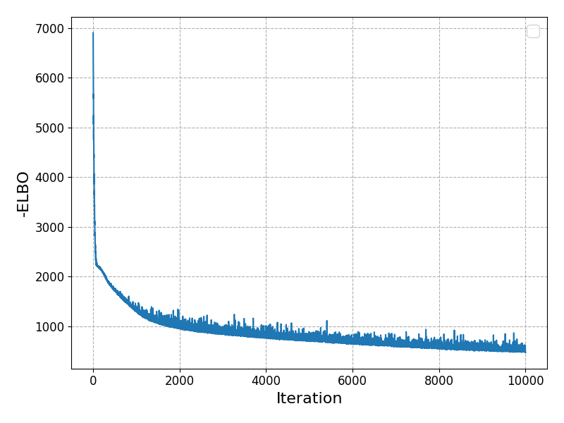
The training loop here is similar to standard backpropagation, but now we optimize the ELBO (actually the negative ELBO since we are performing a minimisation).

Again we define the loss and initialise our variational parameters:

 1
 2
 3
 4
 5
 6
 7
 8
 9
10
11
12
13
14
15
16
17
18
19
20
21
@eqx.filter_jit
def step(params, opt_state, x, y, model_unflatten, key):
    def loss_fn(p):
        return -elbo(p, x, y, model_unflatten, key)
    
    loss_val, grads = jax.value_and_grad(loss_fn)(params)
    updates, opt_state = optimizer.update(grads, opt_state)
    params = optax.apply_updates(params, updates)
    return params, opt_state, loss_val

# Initialize variational parameters
key, subkey = jax.random.split(key)
model = MLP(subkey)
model_arrays, model_static = eqx.partition(model, eqx.is_array)
flat_params, unravel_arrays = ravel_pytree(model_arrays)

# Initialize variational parameters
var_params = VariationalParams(
    mean=flat_params,
    log_std=-4 * jnp.ones_like(flat_params),
)

and build a little training loop

1
2
3
4
5
6
7
8
9
optimizer = optax.adam(1e-3)
opt_state = optimizer.init(var_params)

# More iterations seem to be needed for ELBO optimization (vs 1000 above for standard MSE)
for i in range(10_000):
    key, subkey = jax.random.split(key)
    var_params, opt_state, loss = step(
        var_params, opt_state, x, y, model_unflatten, subkey
    )

we can again check that our loss function has converged well:

BNN MLP training

Making Predictions with Uncertainty

To make predictions, we sample multiple parameter sets and compute statistics:

 1
 2
 3
 4
 5
 6
 7
 8
 9
10
11
12
13
14
15
16
17
18
19
20
def predict_many(var_params, model_unflatten, xx, *, key, n_samples=1000):
    def predict_one(key):
        sample = sample_params(var_params, key)
        model_draw = model_unflatten(sample)
        return jax.vmap(model_draw)(xx).squeeze()
    
    keys = jax.random.split(key, n_samples)
    preds = jax.vmap(predict_one)(keys)  # Shape: [n_samples, n_test_points]
    
    # Compute how much predictions vary due to parameter uncertainty
    mean = preds.mean(axis=0)
    std = preds.std(axis=0)
    return mean, mean - 2 * std, mean + 2 * std

# Make predictions on test range
xx = jnp.linspace(-30.0, 30.0, 400).reshape(-1, 1)
key, subkey = jax.random.split(key)
mean, lower, upper = predict_many(
    var_params, model_unflatten, xx, key=subkey, n_samples=1000
)

Plotting the mean prediction along with the $\pm 2\sigma$ bands shows that the model has been able to learn model parameter uncertainties which describes the data distribution well:

BNN MLP predictions

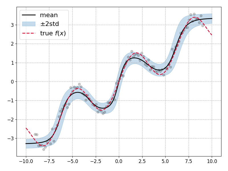
Lovely! Though there are some important caveats to note: The model performance is quite sensitive to several key choices

Observation noise (obs_noise): I’ve somewhat cheated here by using the true observation noise (0.2) in the likelihood calculation within the ELBO. In practice, you’d either need to estimate this from data or treat it as another parameter to infer. The model’s uncertainty estimates are heavily dependent on getting this right.
Initial log standard deviation: The choice of -4 for initial log_std required some manual tuning. Too small and the model becomes overly confident; too large and training became unstable.
Prior variance: I’ve assumed a unit Gaussian prior (prior_std = 1.0) which may not be appropriate for all datasets or models. But in real-life applications we should be standardising our data which should make this choice less egregious.

Summary & Next Steps

This was a short introduction to Variational Inference in which we’ve introduced the concept of a variational approximation family, and used the KL divergence to derive an expression for the Evidence Lower Bound.

With a little tuning we were able to train a Bayesian neural network in which all of our standard model weights and biases were promoted to Gaussian variables parameterised by a mean and standard deviation. We saw how this model performed similarly to a standard neural network, but with the added advantage that we were able to extract prediction uncertainties.

In the next post I’ll introduce the Recursive Variational Gaussian Approximation (finally!). This will combine ideas from this post, and the previous post, to allow us to train non-linear models (neural networks) on streaming data.