Online Bayesian Learning Part 3: R-VGA

Introduction

In part 1, we implemented exact recursive Bayesian updates for linear regression, taking advantage of conjugate priors to derive closed-form posterior updates.

In part 2, we introduced variational inference as a way to approximate intractable posteriors in Bayesian neural networks. Specifically, we can approximate the true posterior $p(\theta|\mathcal{D})$ with a distribution from our chosen ‘variational family’, we chose the family of all Gaussian distributions. In batch variational inference, we optimise the Evidence Lower Bound (ELBO) over the entire dataset to find the parameters $\{\mu, \Sigma\}$ such that our approximation is the best possible fit for the true posterior.

R-VGA extends this to the streaming setting which we saw in part 1, where new data $(X_t, y_t)$ arrives in batches with each timestep $t$. Our choice of a linear Gaussian model with Gaussian priors in part 1 resulted in an exact expression for our posterior but, as in part 2, things are more complicated when we opt for a non-linear neural network.

In this post I’ll follow the derivation from Lambert’s original paper [3] and will reproduce the experiment in section 2.4.4 from [4]. Namely, we’ll build a Bayesian neural network to model a streaming variation of the classic ‘make moons’ binary classification dataset.

A jupyter notebook version of the code in this post is available here.

R-VGA Derivation

The R-VGA algorithm ‘big picture’ is very similar to the story told in part 1: armed with some chosen measurement model and some Gaussian priors:

1. The previous posterior becomes our prior when updating under a new batch of data: $q_{t-1}(\theta) = \mathcal{N}(\mu_{t-1}, \Sigma_{t-1})$. If this is our first batch then we use our initial prior
2. Update the variational parameters: Find new $\mu_t, \Sigma_t$ by optimising the ELBO with respect to the new data
3. Repeat

The update this time is more involved. We start out with an expansion of the KL divergence term, taken verbatim from [3], below.

Letting $Y_t = (y_1, …y_t)$ denote the observations up to, and including time $t$ and take $q_t(\theta)$ to be our variational approximation to the true posterior at time $t$

$$q_t(\theta) = \mathcal{N}(\mu_t, \Sigma_t).$$

Then:

$$\begin{align*} \mathrm{KL}\big(q_t(\theta)|p(\theta\mid Y_t)\big) &= \int q_t(\theta)\log \frac{q_t(\theta)}{p(\theta\mid Y_t)} d\theta \\ &= \int q_t(\theta)\log \frac{q_t(\theta)p(y_t\mid Y_{t-1})}{p(y_t\mid \theta, Y_{t-1})p(\theta\mid Y_{t-1})} d\theta \\ &= \int q_t(\theta)\log \frac{q_t(\theta)p(y_t\mid Y_{t-1})}{p(y_t\mid \theta)p(\theta\mid Y_{t-1})} d\theta \\ &= \int q_t(\theta)\log \frac{q_t(\theta)p(Y_t)}{p(y_t\mid \theta)p(\theta\mid Y_{t-1})p(Y_{t-1})} d\theta. \end{align*}$$

Going line-by-line: we’ve used the definition of the KL divergence, split up $Y_t=(Y_{t-1}, y_t)$ and used Bayes theorem, used our assumption of the conditional independence of our $y_t$ and, lastly, multiplied top and bottom by $p(Y_{t-1})$ and used the definition of conditional probability. So far, so good. Expanded the log term and the integral:

$$\begin{align*} = &\int q_t(\theta)\log q_t(\theta) d\theta - \int q_t(\theta)\log p(y_t\mid \theta) d\theta - \int q_t(\theta)\log p(\theta\mid Y_{t-1}) d\theta \\ & + \int q_t(\theta)\log p(Y_t)d\theta - \int q_t(\theta)\log p(Y_{t-1}) d\theta \end{align*}$$

The last two integrands are independent of $\theta$ so we can extract the logarithms from the integral and in both cases we’re left with an integral over a distribution, yielding $1$:

$$\begin{align*} = &\int q_t(\theta)\log q_t(\theta) d\theta - \int q_t(\theta)\log p(y_t\mid \theta) d\theta - \int q_t(\theta)\log p(\theta\mid Y_{t-1}) d\theta \\ & + \log p(Y_t) - \log p(Y_{t-1}). \end{align*}$$

At this point the first step of the approximation is taken. We approximate that $p(\theta\mid Y_{t-1})\approx q_{t-1}(\theta)$. Lambert proves that if our variational family is conjugate to our likelihood then this approximation incurs the same error as in batch variational inference, and that in linear Gaussian models we recover the Kalman equations as seen in part 1, I won’t recount that in detail here but see [3] for details.

With this approximation we have:

$$\begin{align*} \mathrm{KL}\big(q_t(\theta)|p(\theta\mid Y_t)\big) = &\approx \int q_t(\theta)\log q_t(\theta) d\theta - \int q_t(\theta)\log p(y_t\mid \theta) d\theta \\ &- \int q_t(\theta)\log q_{t-1}(\theta) d\theta + \log p(Y_t) - \log p(Y_{t-1}) \end{align*}$$

and since the final two terms are independent of $\theta$ minimising the KL is equivalent to minimising the following

$$\mathbb{E}_{q_t}\left[\log q_t(\theta) - \log q_{t-1}(\theta) - \log p(y_t\mid \theta)\right].$$

We can do so directly by taking the derivative wrt $\mu$ and $\Sigma$.

$\mu$ first:

$$\begin{align*} \nabla_{\mu_t}\mathbb{E}_{q_t}\left[\log q_t(\theta)-\log q_{t-1}(\theta)-\log p(y_t\mid\theta)\right] \\ =\nabla_{\mu_t}\left(\frac{1}{2}\mu_t^\top \Sigma_t^{-1}\mu_t-\mu_t^\top \Sigma_{t-1}^{-1}\mu_{t-1}\right) - \nabla_{\mu_t}\mathbb{E}_{q_t}\left[\log p(y_t\mid\theta)\right] \\ =\Sigma_t^{-1}\mu_t - \Sigma_{t-1}^{-1}\mu_{t-1}-\nabla_{\mu_t}\mathbb{E}_{q_t} \left[\log p(y_t\mid\theta)\right]=0 \\ \mu_t=\mu_{t-1}+\Sigma_{t-1}\nabla_{\mu_t}\mathbb{E}_{q_t} \left[\log p(y_t\mid\theta)\right] \end{align*}$$

and similarly for $\Sigma$:

$$\begin{align*} \nabla_{\Sigma_t}\mathbb{E}_{q_t} \left[\log q_t(\theta)-\log q_{t-1}(\theta)-\log p(y_t\mid\theta)\right] \\ =\nabla_{\Sigma_t} \left(-\tfrac12\log|\Sigma_t|+\tfrac12\operatorname{Tr}(\Sigma_tP_{t-1}^{-1})\right)-\nabla_{\Sigma_t}\mathbb{E}_{q_t} \left[\log p(y_t\mid\theta)\right] \\ =-\tfrac12 \Sigma_t^{-1}+\tfrac12 \Sigma_{t-1}^{-1}-\nabla_{\Sigma_t}\mathbb{E}_{q_t} \left[\log p(y_t\mid\theta)\right]=0 \\ \Sigma_t^{-1}=\Sigma_{t-1}^{-1}-2\nabla_{\Sigma_t}\mathbb{E}_{q_t} \left[\log p(y_t\mid\theta)\right] \end{align*}$$

These two gradient-of-expectation shaped terms are going to be a nightmare to compute. Happily we can use the following two useful identities (see the appendix of [5] for a proof)

$$\begin{align*} \nabla_{\mu}\mathbb{E}_{q(\theta\mid\mu,\Sigma)}[\log p(y\mid\theta)] &= \mathbb{E}_{q(\theta\mid\mu,\Sigma)}[\nabla_{\theta}\log p(y\mid\theta)] \\ \nabla_{\Sigma}\mathbb{E}_{q(\theta\mid\mu,\Sigma)}[\log p(y\mid\theta)] &= \tfrac{1}{2}\mathbb{E}_{q(\theta\mid\mu,\Sigma)}[\nabla_{\theta}^{2}\log p(y\mid\theta)] \end{align*}$$

and now we have some expectation-of-gradient shaped terms which we can simply compute by approximating the expectation with a sum over samples and using jax.grad and jax.hessian (erm…actually this isn’t true! More on this in a moment).

In summary then, our update terms for R-VGA are:

$$\boxed{ \begin{aligned} \mu_t &= \mu_{t-1} + \Sigma_{t-1}\mathbb{E}_{q_t}\big[\nabla_{\theta}\log p(y_t \mid \theta)\big] \\ \Sigma_t^{-1} &= \Sigma_{t-1}^{-1} - \mathbb{E}_{q_t}\big[\nabla_{\theta}^{2}\log p(y_t \mid \theta)\big] \end{aligned} }$$

R-VGA: Practical consideration…

There are a few sticking points with these we need to think about before we can move to the code…

Implicit vs. explicit schemes

Looking closely at the above update rules we can see that they are only implicitly defined, that is, the new parameters $(\mu, \Sigma)$ are also present on the right hand side, tucked away in the expectation taken over $q_t(\mu, \Sigma)$.

Lambert suggests that we can simply cheat approximate a little further by taking the expectation over a distribution we expect to be close to $q_t(\mu, \Sigma)$ but which we already know, namely, $q_{t-1}(\mu, \Sigma)$. But he acknowledges that the implicit scheme is optimal, under the assumptions and approximations thus far, if we can live with it. While working on the following implementation I tried both and found (1) that the results were very similar and (2) that the performance cost of solving the implicit scheme was tolerable. As a result in the below code example you will see the implicit scheme implemented.

But how do we solve the implicit scheme? Using fixed-point iteration. For each new individual update (i.e. updating $\mu_{t-1}, \Sigma_{t-1}\rightarrow \mu_{t}, \Sigma_{t}$) we perform multiple updates, slowly converging to the true distribution $(\mu_{t}, \Sigma_{t})$. This is, I admit, a little hand-wavey and the code could be made more robust with checks performed on the convergence of our variational parameters, but in practice I found that a small fixed number of fixed-point iterations worked fine.

Computing $\mathbb{E}_{q_t}$

We need to compute two expectations over various derivatives of our model log-likelihood. Lambert’s paper shows that for some simple models such as logistic regression we can perform some pretty impressive gymnastics to compute this expectation without the need for further approximation, but here I have opted to perform a small Monte Carlo estimation for both of these expectation terms. We simply draw a fixed number of parameters from our variational distribution and approximate the expectation integral with a sum.

The Hessian

All of this is getting a bit complicated but as I mentioned above at least we can just use jax’s autodiff to compute the first and second derivative terms for us right? right?

Wrong!

For a non-linear model such as a neural network we aren’t guaranteed that the Hessian will be positive definite, which can (and did, when I didn’t spot this in the implementation!) cause headaches when we come to compute its inverse in the update equations. Instead we can use the Gauss-Newton approximation to the Hessian:

For Bernoulli observations with mean $\mu_i(\beta)$, the log-likelihood is given by

$$\ell(\beta) = \sum_{i=1}^n \Big[ y_i \log \mu_i(\beta) + (1-y_i)\log\big(1-\mu_i(\beta)\big) \Big].$$

The gradient of this is given by

$$\nabla \ell(\beta) = \sum_{i=1}^n \big(y_i - \mu_i(\beta)\big) \frac{\partial \mu_i(\beta)}{\partial \beta},$$

and the second-derivative of the log-likelihood:

$$\nabla^2 \ell(\beta) = -\sum_{i=1}^n \mu_i(\beta)\big(1-\mu_i(\beta)\big) J_i(\beta) J_i(\beta)^\top + \sum_{i=1}^n \big(y_i - \mu_i(\beta)\big) \frac{\partial^2 \mu_i(\beta)}{\partial \beta^2}$$

Two interesting things to note about this expression. (1) The first term is positive semidefinite by construction and (2) the second term is zero in expectation since $\mathbb{E}[y_i-\mu_i]=0$…OK three things, (3) the second term also vanishes if our model is linear since $\frac{\partial^2 \mu_i(\beta)}{\partial \beta^2} = 0$, but that will not be the case for the models under consideration here.

The Gauss-Newton approximation for the Hessian simply drops the second term, leading to a form which is correct in expectation and is positive semidefinite.

R-VGA Implementation

Finally we can actually try out the R-VGA algorithm on some data.

As mentioned in the introduction, I’ve tried to reproduce the experiment from section 2.4.4 Durán-Martín’s thesis [4]. This experiment seeks to model the binary classification ‘make moons’ dataset where batches of randomly sampled data is streamed to us and we are allowed to update our model parameters each time.

The data generating code looks like this:

 1
 2
 3
 4
 5
 6
 7
 8
 9
10
11
12
13
14
15
16
17
18

def make_moons_batch(key, n_per_class=128, noise=0.1):
    key, k0, k1, k_noise = jax.random.split(key, 4)
    θ0 = jax.random.uniform(k0, (n_per_class,)) * jnp.pi
    θ1 = jax.random.uniform(k1, (n_per_class,)) * jnp.pi

    X0 = jnp.stack([jnp.cos(θ0), jnp.sin(θ0)], 1)
    X1 = jnp.stack([1.0 - jnp.cos(θ1), -jnp.sin(θ1) + 0.5], 1)

    X = jnp.concatenate([X0, X1], 0)
    y = jnp.concatenate([jnp.zeros(n_per_class), jnp.ones(n_per_class)], 0)

    X += noise * jax.random.normal(k_noise, X.shape)
    return X, y.astype(jnp.int32), key

def moons_stream(key, T=200, n_per_class=128, noise=0.1):
    for _ in range(T):
        X, y, key = make_moons_batch(key, n_per_class, noise)
        yield X, y

And our Bayesian neural network model will be a simple one-layer MLP. As in previous parts of this mini-series I’m using jax and equinox to implement these models. Part 2 contains some details on the implementation of variational inference using jax/equinox, in case you missed it…

The model then, and some small utilities which will be familiar from last time:

 1
 2
 3
 4
 5
 6
 7
 8
 9
10
11
12
13
14
15
16
17
18
19
20
21
22
23
24
25
26
27
28
29
30

from typing import NamedTuple

import equinox as eqx
import jax
import jax.numpy as jnp
from jax.flatten_util import ravel_pytree


class GaussianPosterior(NamedTuple):
    mean: jax.Array  # (D,)
    covariance: jax.Array  # (D,D)


def tree_to_vec(tree):
    return ravel_pytree(tree)


class MLP(eqx.Module):
    layers: list

    def __init__(self, in_dim, width, key):
        k1, k2 = jax.random.split(key)
        self.layers = [
            eqx.nn.Linear(in_dim, width, key=k1),
            eqx.nn.Linear(width, 1, key=k2),
        ]

    def __call__(self, x):
        h = jax.nn.tanh(self.layers[0](x))
        return self.layers[1](h).squeeze(-1)

The R-VGA update algorithm

 1
 2
 3
 4
 5
 6
 7
 8
 9
10
11
12
13
14
15
16
17
18
19
20
21
22
23
24
25
26
27
28
29
30
31
32
33
34
35
36
37
38
39
40
41
42
43
44
45
46
47
48
49
50
51
52
53
54
55
56
57
58
59
60
61
62
63
64
65
66
67
68
69
70
71
72
73
74

@eqx.filter_jit
def r_vga_update(
    posterior: GaussianPosterior,
    unravel,
    X: jax.Array,
    y: jax.Array,
    *,
    N_fixed_point: int = 10,
    N_monte_carlo: int = 10,
    key,
):
    mu, sigma = posterior
    N_batch, _ X.shape

    def loglik(vec_params):
        net = unravel(vec_params)
        logits = jax.vmap(net)(X)
        logp = -jax.nn.softplus(-logits)
        log1mp = -logits - jax.nn.softplus(-logits)
        return jnp.sum(jnp.where(y, logp, log1mp))

    def logits_fn(v):
        return jax.vmap(unravel(v))(X)

    # Make a 'prequential' prediction: Given our current parameters
    # mu and sigma, predict for the new minibatch (X, y)
    nll_loss = -loglik(mu)
    accuracy = jnp.mean((jax.nn.sigmoid(logits_fn(mu)) >= 0.5) == y)

    D = mu.size

    def fixed_point_itr(carry, key):
        # Sample model parameters via the Cholesky decomposition
        # we do so N_monte_carlo times to estimate the expectations
        # as simple sums
        mu_curr, sigma_curr = carry
        sigma_curr = 0.5 * (sigma_curr + sigma_curr.T)
        jitter = eps * jnp.trace(sigma_curr) / sigma_curr.shape[0]
        L = jnp.linalg.cholesky(sigma_curr + jitter * jnp.eye(D))
        k, key = jax.random.split(key)
        z = jax.random.normal(k, (N_monte_carlo, D))
        theta = mu_curr + z @ L.T

        def gauss_newton_hessian(theta_):
            J = jax.jacrev(logits_fn)(theta_)
            probs = jax.nn.sigmoid(logits_fn(theta_))
            W = probs * (1.0 - probs)
            H_GN = J.T @ (W[:, None] * J)
            return H_GN

        mean_gradient = jax.vmap(eqx.filter_grad(loglik))(theta).mean(axis=0)
        mean_hessian = jax.vmap(gauss_newton_hessian)(theta).mean(axis=0)

        # Update means:
        # N.B. including a scaling factor to get
        # the correct mean update across a batch
        mu_new = mu_curr + sigma_curr @ mean_gradient / N_batch

        # Update covariance:
        lambda_curr = jnp.linalg.inv(sigma_curr + jitter)
        lambda_new = lambda_curr + mean_hessian / N_batch
        sigma_new = jnp.linalg.inv(lambda_new)

        return (mu_new, sigma_new), key

    # Iterate fixed-points using a scan rather than a loop
    keys = jax.random.split(key, N_fixed_point)
    (mu_final, sigma_final), _ = jax.lax.scan(
        fixed_point_itr,
        (mu, sigma),
        keys,
    )

    return GaussianPosterior(mu_final, sigma_final), nll_loss, accuracy

In jax it is usual to express for-loop style logic using a scan. scan allows the ‘carrying’ of state through the ’loop’ which in this case is a tuple of our variational arguments as we move through the fixed point iterations. The second argument is normally some sort of state which is aggregating across loop iterations, but here I’m using it to distribute a jax pseudorandom key to keep all of our sampling independent.

The expectation-of-gradients is happening quite quietly: I’m sampling not one set of parameters for our model at each fixed-point iteration, but N_monte_carlo copies. Then when we need the gradient and hessian of the model for the update we vectorise the computation over the Monte Carlo dimension and take the mean.

Now all we need is a small training loop and we can give it a try:

 1
 2
 3
 4
 5
 6
 7
 8
 9
10
11
12
13
14
15
16

key = jax.random.PRNGKey(0)

net = MLP(in_dim=2, width=32, key=key)
vec0, unravel = tree_to_vec(net)
posterior = GaussianPosterior(vec0, 1.0 * jnp.eye(vec0.size))

X_batches, y_batches, posterior_means, nlls, accuracies = [], [], [], [], []

for X_t, y_t in moons_stream(key, T=300, n_per_class=32, noise=0.2):
    k, key = jax.random.split(key)
    X_batches.append(X_t)
    y_batches.append(y_t)
    posterior, nll, accuracy = r_vga_update(posterior, unravel, X_t, y_t, key=k)
    posterior_means.append(posterior.mean)
    nlls.append(nll)
    accuracies.append(accuracy)

Running this, and looking at the ‘prequential’ (i.e. predict one timestep ahead) negative log-likelihood (NLL) and accuracy we can see that it looks like it’s been able to learn something!

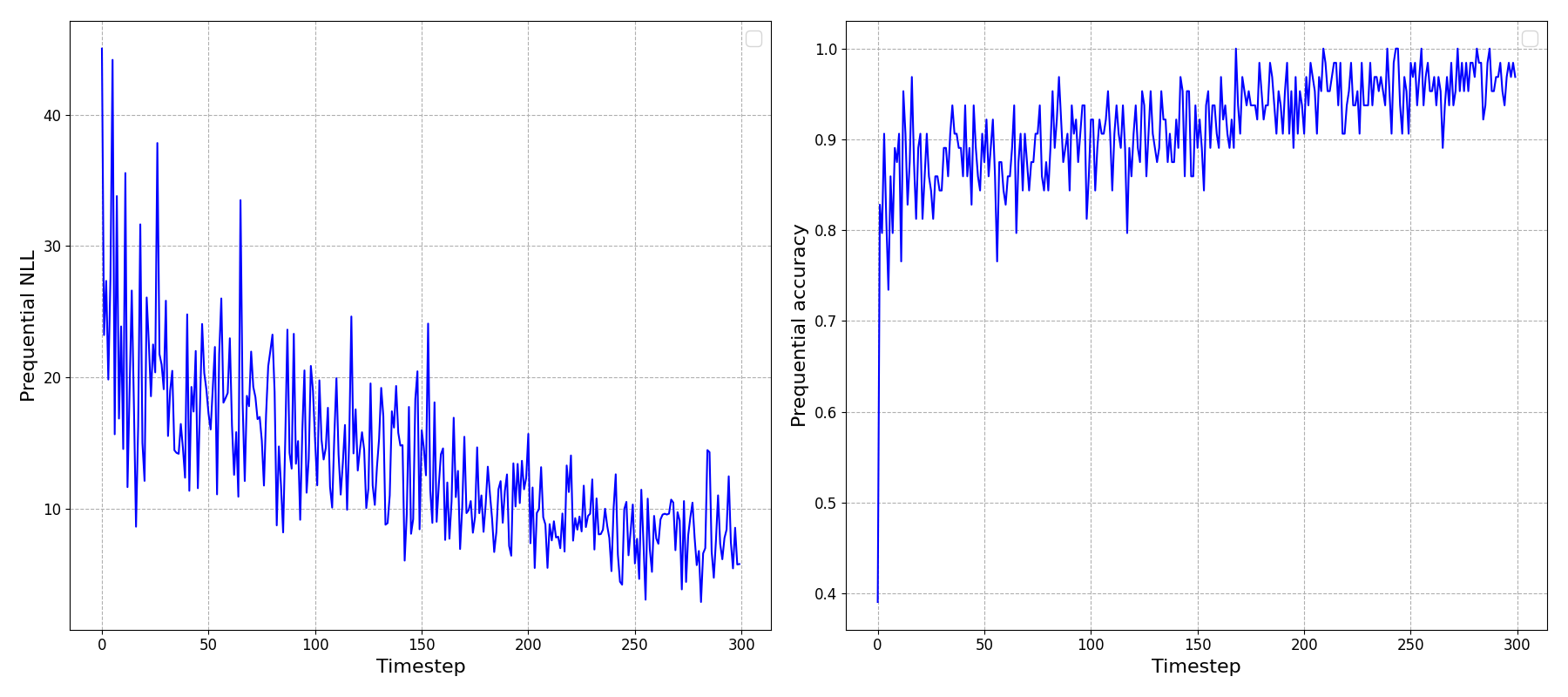
To reinforce an important point here: the $x$-axis above is showing timesteps through our online learning process, not epochs: This is not the usual plot we’ve all seen and made after training a model: we’re not repeatedly showing the model the data and seeing it improve at predicting the full dataset.

Instead, we’re observing the model updating its beliefs after being shown small batches of data at each timestep, and only those data - not the preceding data, and gradually improving its understanding of the underlying dataset. Very cool.

We can also look at the decision boundary learned by the model through time:

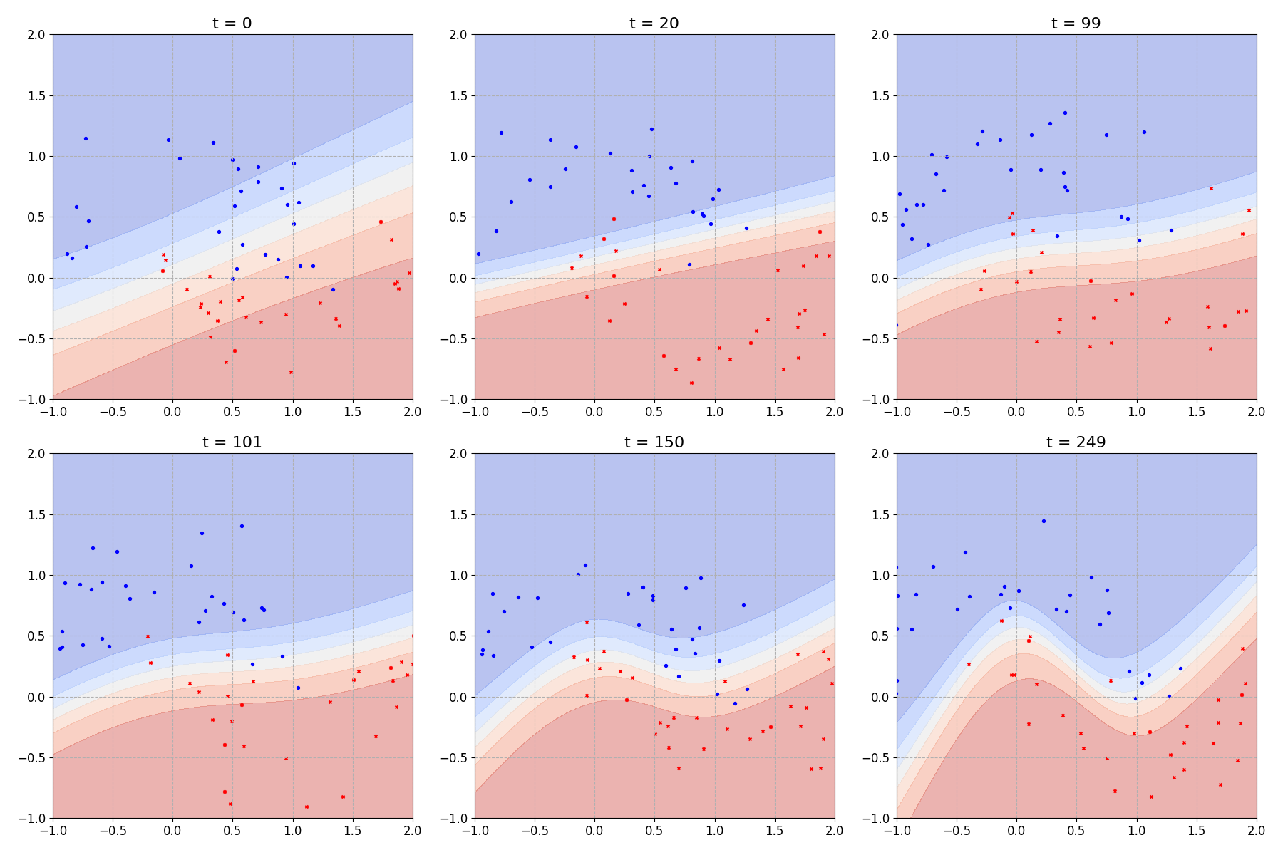
Which looks comparable to figure 2.4 from [4].

In that last plot I chose to plot the mean prediction at each point on the input domain. But our model is still a Bayesian neural network so we could, if we liked, ask it to provide a full prediction distribution for any given point on our input domain.

Summary

In this post, we’ve built on the two previous posts to combine ideas from exact recursive Bayesian inference (Part 1) and variational inference for neural networks (Part 2) in order to implement the Recursive Variational Gaussian Approximation (R-VGA) algorithm.

In the next part, the last part of this mini series, we’ll extend the R-VGA model to describe non-stationary data. Somewhat surprisingly this isn’t as hard as it sounds, the heavy lifting was covered in this post, don’t worry :)

References

[1]: Online Bayesian Learning Part 1: Exact recursive inference

[2]: Online Bayesian Learning Part 2: Bayesian Neural Networks With Variational Inference

[3]: The recursive variational Gaussian approximation (R-VGA) - Lambert et al.

[4]: Adaptive, Robust and Scalable Bayesian Filtering for Online Learning - Gerardo Duran-Martin

[5]: The Variational Gaussian Approximation Revisited - Opper et al.