Online Bayesian Learning Part 4: Non-stationary data and R-VGA

Introduction

In Part 3, we successfully implemented the Recursive Variational Gaussian Approximation (R-VGA) algorithm for online Bayesian learning with neural networks. We demonstrated how R-VGA can learn the two moons classification problem incrementally, updating its beliefs as new data streams arrive.

However, we made a big assumption. We assumed that the underlying data distribution, from which our batches were sampled, remains stationary over time. There are, unfortunately, a lot of real-world modelling problems for which this assumption does not hold. We have to battle seasonal effects, changing markets, changing regulation…the list goes on.

As I promised at the end of Part 3, the heavy mathematical lifting was already done: this post will contain, I think, only one short equation and we’ll be repaid with lots of pretty animations.

A jupyter notebook version of the code in this post is available here.

‘Process noise’

With R-VGA the posterior covariance $\Sigma_t$ ‘shrinks’ with each update, making the model increasingly confident in its current beliefs. This is optimal for stationary data but will probably be very wrong for drifting data.

To model situations where we suspect that the sand (data distribution) is shifting beneath our feet we must generalise our model parameters $\theta_t$ away from being simply our posterior mean after update $t$ and instead view it as a variable in a State Space Model (SSM).

I’m not going to go into SSMs in any detail here (this series has gone on long enough!) but I encourage the interested reader to check out the excellent Särkkä book [7] for the full story.

For our purposes it is sufficient to picture that at each time step we expect to receive a batch of data, and we plan to update our model posteriors in some way (here we’re going to stick with R-VGA). But we now admit some ‘dynamics’ to the system, we explicitly model that from $\theta_{t-1}$ to $\theta_{t}$ some changes will happen. The exact flavour of the changes depend on the sort of SSM we are working with.

In previous posts we’ve used the family of Gaussian distributions as our variational approximation family so we have $\theta = {\mu, \Sigma}$ . Assuming that we don’t have any information about the type of non-stationarity which our data is exhibiting there isn’t much we can say about $\mu$ , so in what follows we will focus on the ‘dynamics’ of $\Sigma$ .

In the Kalman filter literature the model for the dynamics of the underlying quantity of interest is given by the following

$\Sigma_{t}^- = A_{t-1}\Sigma_{t - 1} + q_{t-1}$

where $q_t\sim N(0, Q_t)$ is referred to as the process noise. The $A_t$ matrix allows for linear transformations of our state. The canonical example being that you are trying to estimate the location and velocity of some object through time based on noisy measurements: The velocity directly impacts your understanding of your position, and so you end up constructing an $A_t$ matrix to describe just that.

In our setting $\Sigma_{t}$ obeys no known dynamics, so $A_{t} = I$ . It is also reasonable to claim that our process noise is a constant, since there is no physical process changing through time so we take $Q_t = Q = qI$ . Recall that we are working with a mean field approximation so it makes sense that our process noise is diagonal. These decisions leave us with:

$\Sigma_{t}^- = \Sigma_{t - 1} + qI$

as the ‘predict’ step for our variational covariance. $q\in\mathbb{R}$ is the strength of our process noise.

That’s it, that is all of the maths and (slightly hand wavey) theoretical justification we’ll need to experiment with non-stationary data and the R-VGA algorithm.

The nicest thing about this is that it is very intuitive. R-VGA will tend towards becoming more and more confident, and that confidence is parameterised by the components of $\Sigma$ becoming smaller and smaller as we see more and more data. But we know something that R-VGA does not; we know that $\theta$ is actually changing through time. So, at the start of each update step, we simply explain to R-VGA that there is more uncertainty than it realises, as a result we inflate the covariance matrix a bit and then the rest of the update step proceeds exactly as before.

$q$ is then another hyperparameter of our models we have to tune. Too small and the model will not adapt to new data, too large and it will buy the hype about each new batch of data which arrives and we risk an unstable model which is completely ‘forgetting about’ all past data and fitting to small amounts of noisy data which has just arrived.

Implementation

The function to inflate our covariance is nice and simple:

1
2
3
4
5
def covariance_predict(posterior: GaussianPosterior, q: float):
    mu, sigma = posterior
    Q = (q**2) * jnp.eye(mu.size)
    sigma = sigma + Q
    return GaussianPosterior(mu, sigma)

To test this out I’m going to use the same ‘make moons’ dataset from the previous post. Except that the two moons pattern will gradually rotate around the origin with time, and will experience sudden ‘shocks’ where the whole dataset will rotate $\pi$ radians in one step.

 1
 2
 3
 4
 5
 6
 7
 8
 9
10
11
12
13
14
15
16
17
def moons_stream_rotating_with_shocks(
    key, T=500, n_per_class=32, noise=0.1, drift_deg_per_step=0.3
):
    angle = 0.0
    for t_itx in range(T):
        if t_itx % 100 == 0:
            angle += jnp.pi

        key, k_batch = jax.random.split(key)
        X, y, _ = make_moons_batch(k_batch, n_per_class, noise)

        c, s = jnp.cos(angle), jnp.sin(angle)
        R = jnp.array([[c, -s], [s, c]])
        X = X @ R.T

        yield X, y
        angle += jnp.deg2rad(drift_deg_per_step)

We’ll test different levels of process noise to find the optimal balance between stability and adaptability:

 1
 2
 3
 4
 5
 6
 7
 8
 9
10
11
12
13
14
15
16
17
18
19
20
21
22
23
24
QS = (0.0, 1e-2, 0.05, 0.1, 0.2, 0.5)

prior_var = 5.0

for q in QS:
    key = jax.random.PRNGKey(0)

    net = MLP(in_dim=2, width=32, key=key)
    mu_0, unravel = tree_to_vec(net)
    posterior = GaussianPosterior(mu_0, prior_var * jnp.eye(mu_0.size))

    X_batches, y_batches, posterior_means, nlls, accuracies = [], [], [], [], []

    for X_t, y_t in moons_stream_rotating_with_shocks(
        key, T=250, n_per_class=32, drift_deg_per_step=3.0
    ):
        k, key = jax.random.split(key)
        X_batches.append(X_t)
        y_batches.append(y_t)
        posterior = covariance_predict(posterior, q)
        posterior, nll, accuracy = r_vga_update(posterior, unravel, X_t, y_t, key=k)

        # Result saving code redacted because it's not interesting
        # ...

The results show clear patterns in how different levels of process noise affect adaptation:

q	Mean NLL	Mean Accuracy
0.0	24.366	0.847
0.01	22.551	0.869
0.05	14.045	0.933
0.1	11.406	0.943
0.2	11.681	0.948
0.5	14.989	0.967

The mean negative log-likelihood displays a nice optimal value somewhere around $q=0.1$ while the accuracy, slightly strangely just continues to improve the more twitchy we make our model.

Plotting the prequential accuracy for a few of these values we can see two major differences:

“R-VGA prequential accuracy”

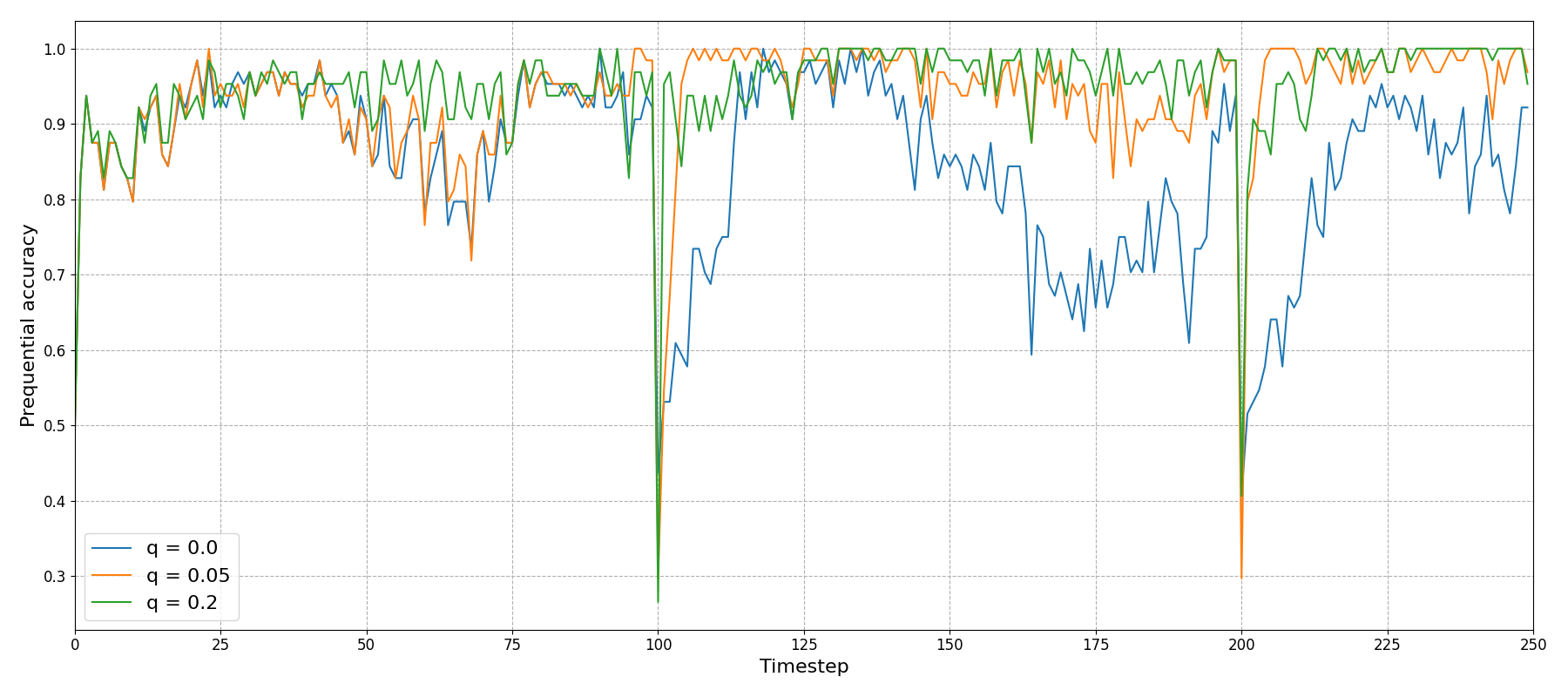
Firstly, and most obviously, the $q=0$ model performs really poorly, as you’d expect for non-stationary data. Even the periods where it appears to rally ( $t\in[200, 225]$ , for example) are actually just times when the data rotates back to a form that the model recognises.

Secondly, There is a clear difference between $q=0.05$ and $q=0.2$ around the ‘shock’ points at $t=100$ and $t=200$ with the larger $q$ value able to much more quickly adjust.

The differences between these choices are even clearer if we look at a little animation of the model trying to keep up with its ever changing landscape:

“R-VGA non-stationary through time”

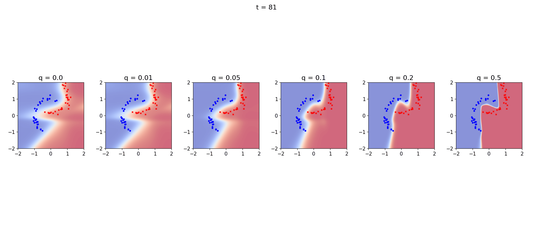
Again we see that the stationary R-VGA completely fails to describe the data, and also that at very high levels of process noise the decision boundaries become non-smooth, I’m not completely sure what is going on there…

Summary

In this final post, we extended R-VGA to handle non-stationary data using a simple but effective technique. By adding a small amount of noise to the covariance matrix we prevent the model from becoming overconfident and enable continued adaptation as data distribution shifts.

Series conclusion: We’ve built a complete framework for online Bayesian learning, progressing from exact conjugate updates (Part 1), introduced the concept of Variational Inference (Part 2), combined these ideas to build an implementation of the R-VGA algorithm which allowed us to describe non-linear, and now non-stationary non-linear data, in a streaming/online fashion.