Building Non-Standard Regression Models with JAX

Introduction

In this post, I’ll show how JAX’s automatic differentiation makes it straightforward to train ’non-standard’ regression models. We’ll implement a Zero-Inflated Generalised Poisson (ZIGP) regression model. This would be tricky to implement from scratch but becomes manageable when we can just formulate the model we are interested in, write down the likelihood and let JAX handle the gradients.

The example comes from the paper “Zero-Inflated Generalized Poisson Regression Model with an Application to Domestic Violence Data” (apologies for the unpleasant subject matter, it just so happened that such a model had been used to describe this data, and the data had been made public which made for a nice reproduction). The model is interesting because we have to deal with both over-dispersion and a zero-inflation component. The inclusion of both of which, as we will see, are important.

A jupyter notebook version of the code in this post is available [5].

The Problem: Count Data with Structural Zeros

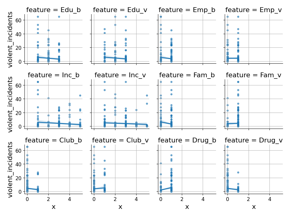
The dataset contains incident counts, $y_i$, from households, along with covariates, $X_{ij}$, which are answers to a series of survey questions which the surveyors presumably thought were likely to be correlated with the rate of incidence.

This type of data exhibits three key features that make standard Poisson regression inadequate:

• Structural zeros: Many survey responses have $y_i = 0$, more than would be expected from a standard count distribution. Some of these zeros are ‘structural’ (households where incidents would never occur) but some are ‘sampling’ zeros ($y_i > 0$ was possible in principle but this was not observed).
• Over-dispersion: The variance in incident counts substantially exceeds the mean, violating the Poisson assumption that mean equals variance.
• Regression structure: We have covariates for both the the zero-inflation process and the ‘base’ count process (Poisson, Generalised Poisson, …).

We can inspect the interactions of each feature and the dependent variable to get a rough idea of what the relationships might look like:

The ZIGP Model

The Zero-Inflated Generalised Poisson (ZIGP) model meets, exactly, the demands of this dataset. It models count data, which may or may not have experience zero inflation (ZI), using a Generalised Poisson distribution (GP).

The Generalised Poisson Distribution

The standard Poisson distribution assumes $\text{Var}(Y) = \mathbb{E}[Y]$ but this is often violated in practice. The Generalised Poisson relaxes this constraint by introducing a dispersion parameter $\alpha$, giving a PMF of:

$$P(Y = y | \lambda, \alpha) = \frac{\lambda^y(1+\alpha y)^{y-1}e^{-\lambda(1+\alpha y)}}{y!}$$

with mean $\mathbb{E}[Y] = \lambda/(1-\alpha\lambda)$. When $\alpha > 0$, the distribution exhibits over-dispersion ($\text{Var}(Y) > \mathbb{E}[Y]$), while $\alpha < 0$ gives under-dispersion. As $\alpha \to 0$, we recover the standard Poisson distribution.

Zero-Inflation Component

To handle structural zeros, we add a mixture component using a Bernoulli model for the probability $\phi_i$ that observation $i$ is a structural zero. Although there are other links which could be experimented with, the logistic link is natural here and provides a smooth, interpretable mapping from covariates to probabilities.

Full ZIGP Specification

Combining these ideas we have, for observation $i$, the following PMF:

$$P(Y_i = y_i) = \begin{cases} \phi_i + (1-\phi_i)e^{-\lambda_i} & \text{if } y_i = 0 \\ (1-\phi_i)\frac{\lambda_i^{y_i}(1 + \alpha y_i)^{y_i-1}e^{-\lambda_i(1+\alpha y_i)}}{y_i!} & \text{if } y_i > 0 \end{cases}$$

where $\phi_i$ is the probability of a structural zero, $\lambda_i$ is the Poisson rate parameter and $\alpha$ is the dispersion parameter.

Now we follow the regression structure from [1]:

$$\begin{align*} \mu_i &= \exp(X_i^\top\beta) \\ \phi_i &= \sigma(X_i^\top\gamma) \end{align*}$$

where $\beta, \gamma \in\mathbb{R}^D$.

The authors make the choice to couple the Generalised Poisson mean, $\mu_i$, and the zero-inflation parameter, $\phi_i$, by introducing a parameter $\tau\in\mathbb{R}$, and taking $\beta = -\tau \gamma$. Intuitively this makes some sense: the zero inflation increases as the mean decreases. However, it is not entirely clear to me that this is the optimal because we do not know that structural zeros are being ‘generated’ by the same process as the sampled zeros…Indeed I thought that was sort of the crux of the model! Possibly the authors tried using uncoupled regression designs for the Generalised Poisson component and the Zero Inflation component and found that either it didn’t converge well or that it wasn’t possible to derive the update steps required in this case. Either way, in what follows I will follow in their footsteps with the aim of reproducing their results.

Implementation

This is one of the reasons JAX is so useful. Instead of deriving the gradient by hand (which can be done, as in [1]), we simply implement the negative log-likelihood:

 1
 2
 3
 4
 5
 6
 7
 8
 9
10
11
12
13
14
15
16
17
18
19
20
21
22
23
24
25
26
27
28
29
30
31
32
33
34
35

def zipg_unpack_theta(theta, p):
    beta = theta[:p]
    tau = theta[p]
    gamma = theta[p + 1]
    return beta, tau, gamma


def zigp_neg_loglik_coupled(theta, X, y):
    _, p = X.shape
    beta, tau, gamma = zipg_unpack_theta(theta, p)

    mu = jnp.exp(X @ beta)
    phi = jax.nn.sigmoid(-tau * X @ beta)

    alpha = jax.nn.softplus(gamma) + eps_alpha
    lambda_ = mu / (1.0 + alpha * mu)

    y = y.astype(jnp.int64)
    is_zero = y == 0
    is_pos = y > 0

    ll_zero = jnp.log(phi + (1.0 - phi) * jnp.exp(-lambda_))
    y_pos = y[is_pos]
    lambda__pos = lambda_[is_pos]
    phi_pos = phi[is_pos]
    term_pos = (
        jnp.log1p(-phi_pos)
        + y_pos * jnp.log(lambda__pos)
        + (y_pos - 1.0) * jnp.log1p(alpha * y_pos)
        - jax.scipy.special.gammaln(y_pos + 1.0)
        - lambda__pos * (1.0 + alpha * y_pos)
    )

    ll = jnp.sum(ll_zero[is_zero]) + jnp.sum(term_pos)
    return -ll

The implementation follows the mathematics closely:

1. We unpack $\theta$ into $\beta$ (regression coefficients), $\tau$ (zero-inflation scaling), and $\gamma$ (transformed dispersion parameter)
2. Compute $\mu_i = \exp(X_i^\top\beta)$ and $\phi_i = \sigma(-\tau \cdot X_i^\top\beta)$
3. Transform $\gamma \to \alpha$ via softplus to ensure $\alpha > 0$
4. Calculate the rate parameter $\lambda_i = \mu_i / (1 + \alpha\mu_i)$

With that in hand, training the model is straightforward: We simply use scipys implementation of L-BFGS-B with JAX’s autograd providing the gradient.

 1
 2
 3
 4
 5
 6
 7
 8
 9
10
11
12
13
14
15
16
17
18

def loss(theta_):
    return zigp_neg_loglik_coupled(theta_, X, y)

def grad(theta_):
    return jax.grad(loss)(theta_)

theta0 = jnp.zeros(p + 2)

result = minimize(
    loss,
    theta0,
    method="L-BFGS-B",
    jac=grad,
    options={"disp": True, "maxiter": 100},
)

theta_zigp = result.x
zigp_nll = result.fun

We can also train two simpler (nested) models for comparison:

1. a standard Poisson (by fixing $\tau = \gamma = -10$, effectively setting $\phi \approx 0$ and $\alpha \approx 0$) and
2. a Generalised Poisson without zero-inflation by fixing only $\tau = -10$.

Results

At convergence the model has the following parameter estimates:

Which matches the ZIGP coefficients from [1] well.

Approximate Parameter Uncertainty

To perform inference on the results of the study we need uncertainties on these point-values. Drug_b looks to be quite strongly correlated with incidence, but if we were told that the error on this value is $\pm 2$ it changes the picture completely.

We can get these uncertainty bounds approximately, even for a reasonably fancy model like the ZIGP, for free with the code we’ve already written.

This is a fundamental result in asymptotic statistics [3]. Let $\ell(\theta) = \sum_{i=1}^n \log p(y_i | \theta)$ be the log-likelihood. The score function is:

$$s(\theta) = \nabla \ell(\theta)$$

Taylor expanding the score around the true parameter $\theta_0$ up to the second order term

$$0 = s(\hat{\theta}) \approx s(\theta_0) + H(\theta_0)(\hat{\theta} - \theta_0)$$

where $H(\theta) = \nabla^2 \ell(\theta)$ is the Hessian. The linear term is zero because at the MLE, $\hat{\theta}$, we have $s(\hat{\theta}) = 0$. Rearranging this:

$$\sqrt{n}(\hat{\theta} - \theta_0) \approx -H(\theta_0)^{-1} \sqrt{n} s(\theta_0)$$

Under regularity conditions:

1. The score satisfies a central limit theorem: $\sqrt{n} s(\theta_0) \rightarrow N(0, \mathcal{I}(\theta_0))$, where $\mathcal{I}(\theta) = \mathbb{E}[-H(\theta)]$ is the Fisher information
2. The Hessian converges: $H(\theta_0) / n \rightarrow -\mathcal{I}(\theta_0)$

Therefore:

$$\sqrt{n}(\hat{\theta} - \theta_0) \rightarrow N\left(0, \mathcal{I}(\theta_0)^{-1}\right)$$

In practice, we replace the expected Fisher information $\mathcal{I}(\theta_0)$ with the observed information $-H(\hat{\theta})$, giving us:

$$\hat{\theta} \sim N\left(\theta_0, [-H(\hat{\theta})]^{-1}\right)$$

Since we’re minimizing the negative log-likelihood, our Hessian is already positive, so $\text{Cov}(\hat{\theta}) \approx H^{-1}$.

JAX’s automatic differentiation makes it straightforward to compute approximate standard errors using the Hessian:

 1
 2
 3
 4
 5
 6
 7
 8
 9
10
11

H = jax.hessian(loss)(theta_zigp)
ridge = 1e-8
H_pd = H + ridge * jnp.eye(H.shape[0])
cov = jnp.linalg.inv(H_pd)
se = jnp.sqrt(jnp.diag(cov))

z_scores = theta_zigp / se
p_values = 2 * (1 - norm.cdf(np.abs(z_scores)))

ci_lower = theta_zigp - 1.96 * se
ci_upper = theta_zigp + 1.96 * se

Again, these match the results from [1] well.

Zero-inflation is significant: The $\gamma$ parameter is highly significant (p < 0.001), which we interpret as the zero-inflation component contributing towards the model.

With $\hat{\gamma} = -1.03$, we get $\hat{\alpha} = \text{softplus}(-1.03) \approx 0.36$, so there is a reasonable degree of over-dispersion in the data. The $2\sigma$ lower bound on $\alpha$ is $\text{softplus}(-1.445) \approx 0.21$ so it is also ‘significant’ for over-dispersion.

Drug problems strongly predict incidence: Having drug problems at baseline (Drug_b) is the strongest predictor, associated with exp(1.54) ≈ 4.7× higher incident rates.

Education and social engagement matter: Higher education at visit (Edu_v) and club membership at baseline (Club_b) are both associated with significantly lower incidence rates.

Income shows positive association at visit: Contrary to expectations, income at visit (Inc_v) shows a positive association with incident counts, though this could reflect reporting bias or other confounding.

Model Comparison

To validate that the ZIGP model is truly necessary, we compare it against two simpler ’nested’ models using information criteria and likelihood ratio tests:

The ZIGP model outperforms both alternatives. The standard Poisson model looks misspecified (Δ_AIC > 3500), while even the Generalised Poisson—which handles over-dispersion—is substantially worse than ZIGP (Δ_AIC ≈ 129).

Likelihood ratio tests confirm these findings:

1. Poisson vs Generalised Poisson: LR = 3562.23, p < 0.001 → Reject Poisson; over-dispersion is real

2. Generalised Poisson vs ZIGP: LR = 130.95, p < 0.001 → Reject GenPoisson; zero-inflation is necessary

3. Poisson vs ZIGP: LR = 3693.18, p < 0.001 → Strongly reject simplest model

All tests overwhelmingly reject the simpler models, confirming that both over-dispersion and zero-inflation are essential features of this data.

Summary

In this post we implemented a Zero-Inflated Generalised Poisson regression model to analyse domestic violence incident data. We were able to reproduce the results found by the authors of [1], but without having to worry about manually compute gradients of our arbitrarily complicated likelihood.

Similarly we saw that JAX can provide Hessians for our models in a single line of code, enabling us to provide approximate uncertainty bounds for our regression coefficients.

The combination of mathematical flexibility and computational efficiency makes custom model development accessible to anyone comfortable with numpy…sort of - JAX does have some self-confessed “sharp bits” to avoid [4]!

References

[1] Famoye, F., & Singh, K. P. (2006). Zero-Inflated Generalized Poisson Regression Model with an Application to Domestic Violence Data . Journal of Data Science, 4(1), 117-130.

[2] JAX: Composable transformations of Python+NumPy programs . Google Research.

[3] Casella, G., & Berger, R. L. (2002). Statistical Inference (2nd ed.). Duxbury Press. Chapter 10: Asymptotic Evaluations.

[4] JAX's 'sharp bits'

[5] Notebook