Intro to robustness: optimality and feasibility

In the next few posts I’m going to work through a paper by Bertsimas and Sim [1] which looks at an interesting approach to making robust decisions using mixed integer linear programmes when dealing with uncertainty in training data. In particular I’ll solve the ‘Knapsack Problem’ in three different ways and then discuss the trade-off: how can we best balance the optimality of our solutions with their feasibility?

In this post I’ll start by briefly introducing the Knapsack Problem and then looking at Soyster’s method for dealing with uncertainty. In the subsequent one or two posts I’ll derive the Bertsimas and Sim model and implement it in gurobi.

The Knapsack Problem

The Knapsack problem is the following simple task: Choose to fill our bags (‘knapsacks’) indexed by \(j\) from a set of available objects indexed by \(i\). Each object has with it an associated value, \(c_i\), and a ’nominal’ weight, \(w_i\). We want to maximise the total value of objects in our bags while not exceeding the weight limits of each, \(l_j\):

$$ \begin{align*} &\max \sum_{i,j} x_{ij} c_i\newline&\text{subject to:}\quad \sum_i x_{ij}w_i\leq l_j \end{align*} $$

where \(x_{ij}\in\{0, 1\}\) are our binary decision variables which indicate if we have chosen to take item \(i\) in knapsack \(j\).

If instead we solved the relaxation \(0\leq x_{ij}\leq 1\) that is known as the continuous knapsack. I’ll focus on solutions to the binary (or zero-one) knapsack problem although the code presented supports both.

Expressing this with the gurobi optimiser is straightforward. Starting with a definition of our problem:

 1
 2
 3
 4
 5
 6
 7
 8
 9
10
11
12
13
14
15
16
17
18
19
20
class KnapsackType(Enum):
    ZERO_ONE = 1
    CONTINUOUS = 2

@dataclass
class PackItem:
    weight: float
    value: float

@dataclass
class Knapsack:
    weight_limit: float

@dataclass
class KnapsackProblem:
    n_items: int
    n_knapsacks: int
    item_list: List[PackItem]
    knapsacks: List[Knapsack]
    type_: KnapsackType

A method to generate example problems to solve (’nominal’ here indicates we are dealing with a single value for the weight of each item, with no uncertainty):

 1
 2
 3
 4
 5
 6
 7
 8
 9
10
11
12
13
14
15
16
17
18
19
20
21
22
23
24
25
26
27
28
29
30
31
32
# The number of items in each problem
N = 200

# The number of knapsacks in each problem
K = 1

ALLOWED_WEIGHTS = np.arange(20, 30)
ALLOWED_VALUES = np.arange(16, 78)
WEIGHT_LIMIT = 4_000


def generate_nominal_problem(
    n_items: int,
    n_knapsacks: int,
    type_: KnapsackType = KnapsackType.ZERO_ONE
) -> KnapsackProblem:
    weights = np.random.choice(ALLOWED_WEIGHTS, size=n_items, replace=True)
    values = np.random.choice(ALLOWED_VALUES, size=n_items, replace=True)
    item_list = [
        PackItem(w, v) for w, v in zip(weights, values)
    ]
    knapsacks = [
        Knapsack(WEIGHT_LIMIT)
        for _ in range(n_knapsacks)
    ]
    return KnapsackProblem(
        n_items,
        n_knapsacks,
        item_list,
        knapsacks,
        type_
    )

and a gurobipy model to find:

  1. the optimal knapsack allocation for a given problem,
  2. the objective value (in our case, the total value of the items)
  3. details of which items were allocated to each knapsack (which will come in handy later for checking the feasibility of our solutions in various settings)
 1
 2
 3
 4
 5
 6
 7
 8
 9
10
11
12
13
14
15
16
17
18
19
20
21
22
23
24
25
26
27
28
29
30
31
32
33
34
35
36
37
38
39
40
41
42
43
44
45
46
47
48
49
50
51
52
53
54
55
56
57
58
59
60
61
62
63
64
65
66
67
68
def create_model(name: str) -> lp.Model:
    m = lp.Model(name)
    m.setParam(lp.GRB.Param.LogToConsole, 0)
    return m


def get_vtype_for_knapsack(type_: KnapsackType):
    return (
        lp.GRB.CONTINUOUS
        if type_ == KnapsackType.CONTINUOUS else
        lp.GRB.BINARY
    )

def optimise_knapsack_model(problem: KnapsackProblem) -> Tuple[np.array, double]:
    m = create_model("KnapsackProblem")

    # allocs[i, j] == 1 -> item i has been placed in knapsack j
    allocs = m.addVars(
        problem.n_items,
        problem.n_knapsacks,
        vtype=get_vtype_for_knapsack(problem.type_),
        ub=1.0,
        name="allocs"
    )

    # Maximise the total value of items selected
    m.setObjective(
        lp.quicksum(
            allocs[i, j] * item.value
            for i, item in enumerate(problem.item_list)
            for j, _ in enumerate(problem.knapsacks)
        ),
        sense=lp.GRB.MAXIMIZE
    )

    # Each item can only be in one knapsack
    m.addConstrs(
        (
            lp.quicksum(allocs[i, j] for j, knapsack in enumerate(problem.knapsacks)) <= 1
            for i in range(problem.n_items)
        ),
        name="one_knapsack_per_item"
    )

    # Each knapsack has a weight limit
    m.addConstrs(
        (
            lp.quicksum(
                allocs[i, j] * problem.item_list[i].weight for i in range(problem.n_items)
            ) <= problem.knapsacks[j].weight_limit
            for j in range(problem.n_knapsacks)
        ),
        name="knapsack_weight_limits"
    )

    m.optimize()

    assert m.status == lp.GRB.OPTIMAL

    allocations = np.array(
        [
            allocs[i, j].X
            for i in range(problem.n_items)
            for j in range(problem.n_knapsacks)
        ]
    ).reshape(problem.n_items, problem.n_knapsacks)

    return allocations, m.ObjVal

And giving it a quick test run…

1
2
3
4
5
6
p = generate_nominal_problem(200, 3)
_, nominal_optimal_value = optimise_knapsack_model(p)

nominal_optimal_value

>>> 9216.0

Good. This should solve extremely fast and the model will, I believe, be small enough to run on the free gurobipy license.

Now moving on to the more interesting stuff.

Uncertainty in our constraint matrix

To describe the situation where we have uncertainty in our weights I will follow the language in [1].

We assume that each entry of our weight constraint matrix, \( \tilde w_{ij}\), is a random variable which can assume values around the ’nominal’ value, \(w_{ij}\), as follows:

$$ \tilde w_{ij} \in [w_{ij} − \hat w_{ij} , w_{ij} + \hat w_{ij}]. $$

For what follows it will also be useful to define:

$$ \eta_{ij} = \frac{(\tilde w_{ij} − w_{ij})}{\hat w_{ij}}, $$

which, by construction, is a symmetric distribution satisfying \(\eta_{ij} = [−1, 1]\).

Soyster’s approach & Murphy’s Law

In Soyster’s paper of 1973 [3] he phrased this problem by considering each weight variable to have a set of possible values and then expanding out the total weight constraint into every combinatorial realisation giving every variable, \(w_i\), its minimum and maximum possible value.

This is the Operational Research version of Murphy’s Law - we are looking at all possible cases and then will focus solely on the ‘worst’ possible scenario. In our case the ‘worst’ case is the one where all of the objects we decide to pick will be at their maximum allowed weight value. It’s going to be extremely conservative which will lead to two important properties of the solutions it finds:

  1. The good news: The solution we choose will always remain feasible no matter what weights are drawn for the random variables - whatever plan we come up is provably going to work out!
  2. The bad news: It’s highly likely that when we know the realised weights of the objects we’ll find out that our plan was way too conservative and this has led us to a solution which is less valuable than it might have been.

The proof of the feasibility again comes from [1]. Start by expanding out the constraint term in terms of \(w_{ij}\) and \(\hat{w}_{ij}\) decomposition:

$$ \sum_j x_j\tilde w_{ij} = \sum_j x_j(w_{ij} + \eta\,\hat{w}_{ij}) \leq l_i $$

$$ \sum_j x_jw_{ij} + \sum_jx_j\eta\,\hat{w}_{ij} \leq l_i $$

Now comes the Soyster ‘worst case’; in place of the \(x_j\,\eta\) term we introduce a new variable \(y_j \geq 0\) which we bound to be greater in magnitude than \(x_j\):

$$ -y_j \leq x_j \leq y_j $$

Leaving our constraint term as

$$ \sum_j x_jw_{ij} + \sum_jy_j\hat{w}_{ij} \leq l_i. $$

Although it looks like we’re allowing the magnitude of the error to be larger than that allowed by the \(|\eta|\leq 1\) constraint we will find that at optimality the constraint linking \(x_j\) and \(y_j\) will be ’tight’ i.e. we will have \(y_j^*=|x_j^*|\) (when an asterisk denotes the value for the corresponding variable once the MIP has been solved to optimality).

It’s easy to show that the optimal values to this Soyster problem will remain feasible for any realisation of the weights of the objects:

$$ \sum_j \tilde w_{ij}x_j^* = \sum_j w_{ij}x_j^* + \sum_j \eta_{ij}\hat{w}_{ij}x_j^* $$

$$ \leq \sum_j w_{ij}x_j^* + \sum_j |x_j^*|\hat{w}_{ij} $$

$$ = \sum_j w_{ij}x_j^* + \sum_j y_j\hat{w}_{ij} \leq l_i $$

Solving the Soyster problem

To demonstrate these good news/bad news properties we can take a nominal problem with some weight uncertainty, and generate the Soyster version of our problem, which optimise_knapsack_model can solve:

 1
 2
 3
 4
 5
 6
 7
 8
 9
10
11
12
13
14
15
16
17
18
19
20
21
22
23
def generate_new_problem(
    nominal_problem: KnapsackProblem,
    weight_updater: Callable
) -> KnapsackProblem:
    new_problem = deepcopy(nominal_problem)
    for item in new_problem.item_list:
        item.weight = weight_updater(item.weight)
    return new_problem

def generate_soyster_weight(
    nominal_weight: float,
    weight_uncertainty: float
) -> float:
    return nominal_weight * (1 + weight_uncertainty)

def generate_soyster_problem(
    nominal_problem: KnapsackProblem,
    weight_uncertainty: float = 0.1
) -> KnapsackProblem:
    return generate_new_problem(
        nominal_problem,
        lambda p: generate_soyster_weight(p, weight_uncertainty)
    )

We can also use the definitions of the random weight variables to generate realisations which deviate from the nominal problem. In this way we can compare objective values of the Soyster formulation with ‘reality’ and also check to see how often our ’nominal’ and Soyster solutions remain feasible once we know the actual weights of the knapsack items:

 1
 2
 3
 4
 5
 6
 7
 8
 9
10
11
12
13
14
15
16
17
18
19
20
21
22
23
24
25
26
27
28
29
30
31
32
33
34
35
36
37
38
39
40
41
42
43
44
45
46
47
48
49
50
51
52
53
54
55
56
57
58
59
60
61
62
63
64
65
66
67
68
69
70
71
72
def generate_random_weight(
    nominal_weight: float,
    weight_uncertainty: float
) -> float:
    return nominal_weight * (1 + np.random.uniform(-weight_uncertainty, weight_uncertainty))

def generate_random_problem(
    nominal_problem: KnapsackProblem,
    weight_uncertainty: float = 0.1
) -> KnapsackProblem:
    return generate_new_problem(
        nominal_problem,
        lambda p: generate_random_weight(p, weight_uncertainty)
    )

def is_allocation_feasible(
    item_list: List[PackItem],
    allocs: np.array,
    weight_limit: float
) -> bool:
    return all(
        np.array([
            sum([
                item.weight * alloc
                for item, alloc in zip(item_list, allocs[:, k])
            ])
            for k in range(K)
        ]) <= weight_limit
    )

def simulate_soyster_vs_realised_problems(
    nominal_problem: KnapsackProblem,
    n_trials: int
) -> Tuple[float, np.array, np.array]:
    # Compute Soyster's view on this problem and optimise it:
    soyster_problem = generate_soyster_problem(nominal_problem)
    soyster_allocs, soyster_optimal_value = optimise_knapsack_model(soyster_problem)

    realised_optimal_values = []
    realised_feasibility = []
    soyster_feasibility = []

    for _ in range(n_trials):
        # Draw realised weights from the nominal problem and optimise it
        random_problem = generate_random_problem(nominal_problem)

        # Soyster is always feasible...but check it all the same:
        soyster_feasibility.append(
            is_allocation_feasible(random_problem.item_list, soyster_allocs, WEIGHT_LIMIT)
        )

        # Find the realised optimal and see if the nominal solution
        # remained feasible
        random_allocs, realised_optimal_value = optimise_knapsack_model(random_problem)
        realised_optimal_values.append(realised_optimal_value)
        realised_feasibility.append(
            is_allocation_feasible(nominal_problem.item_list, random_allocs, WEIGHT_LIMIT)
        )

    return (
        soyster_optimal_value,
        np.array(realised_optimal_values),
        np.array(realised_feasibility),
        np.array(soyster_feasibility),
    )

(
    soyster_optimal_value,
    realised_optimal_values,
    realised_feasibility,
    soyster_feasibility,
) = simulate_soyster_vs_realised_problems(p, 500)
1
2
3
4
5
>>> realised_feasibility.mean()
0.342

>>> soyster_feasibility.mean()
1.0

Soyster vs. Realised Objective Values

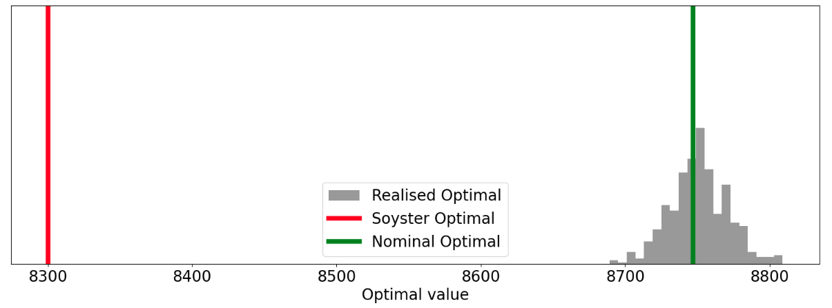
We can see that every realised set of weights is feasible under the Soyster solution but that if we just optimised assuming the mean weights our plan only remained valid 34.2% of the time! We can also see from the distribution of realised optimal values that the Soyster solution is leaving a not insignificant amount of value on the table…Is there a way we can trade off these two goals in a more graceful way?

Yes (obviously)! In the next post, or two, I’ll continue on and derive the more flexible Bertsimas and Sim alternative.

References

[1]: The Price of Robustness - Bertsimas and Sim

[2]: Theory and applications of Robust Optimization - Bertsimas et. al.

[3]: Convex Programming with Set-Inclusive Constraints and Applications to Inexact Linear Programming - Soyster

[4]: Data-Driven Robust Optimization Using Scenario-Induced Uncertainty Sets - Cheramin et. al.