Bivariate Poisson Regression with Expectation-Maximisation

Count data is commonly modelled using a generalised linear model with a Poisson likelihood, and this approach extends trivially to cases with multiple count data random variables, $Z_i\in {\mathbb{Z}}^{0+},i=1\dots N$ which are indepedent of one another, $Z_i\perp Z_j,\mathrm{\forall }i,j$ because the likelihoods factor out nicely. But what about the case where there is some correlation?

In this short post I’ll describe the case in which we have two correlated count variables and we believe that a linear function of some known covariates can explain variation in the data.

Univariate Poisson regression and the MLE fit

The poisson distribution is specified by a parameter, ${\lambda }_i\in \mathbb{R}$, which turns out to be both its mean and variance. It’s PMF for an observation, $z_i$, is given by

$$\text{Po}(z_i|{\lambda }_i)=\frac{{\lambda }_i^{z_i}{e}^{-{\lambda }_i}}{z_i!}.$$

Assuming the data is IID then the log-likelihood is given by:

$$\mathcal{L}({\lambda }_i|z_i)=\sum _i^n{z}_i\log ({\lambda }_i)-{\lambda }_i-\log (z_i!).$$

The last piece we need, a ’link function’: There are a couple of options we can use to relate the Poisson parameter to our model parameters, ${\beta }_j$, and the observed covariates, $z_j$, but the common choice is the log-link:

$$\log {\lambda }_i=\overrightarrow{\beta }\cdot \overrightarrow{x_i}$$

Typically we would take derivatives of the log-likelihood with respect to the $w_j$ using the chain rule and use the iteratively reweighted least squares algorithm (see page 294 of ¹ for details on that approach) but here we can be lazy and let scipy’s brentq minimisation do the hard work for us (this will require more function evaluations than if we provided the derivative of the negative log-likelihood and prefered L-BFGS over brentq, but everything here runs in O(seconds) on a laptop for me anyway…)

We’re nearly ready to start fitting some models, but first some housekeeping to make our life easier later:

from dataclasses import dataclass
from typing import TypeVar, Generic, Tuple, Union, Optional
import numpy as np
import pandas as pd
from scipy import optimize

@dataclass
class Dims:
    N: int
    M: int

@dataclass
class ObservedData:
    covariates: np.array
    Z0: np.array
    Z1: np.array = None

@dataclass
class PoissonData:
    dims: Dims
    observed: ObservedData

We can generate some fake data from a true model lambdas by generating some random covariates and using some true model $\beta$’s, and then sampling from the resulting Poisson distributions:

def generate_poisson_data(true_betas: np.array, N: int, sigma=1) -> PoissonData:
    M = true_betas.shape[0]
    covariates = np.random.normal(0, sigma, (N, M))
    # Fix the first row to allow for a constant term in the regression
    covariates[0, :] = 1
    lambdas = np.exp(covariates.dot(true_betas))
    poisson_draws = np.random.poisson(lambdas)
    return PoissonData(Dims(N, M), ObservedData(covariates, poisson_draws))

and, as above, in order to fit the model we need an expression for the negative (so make the problem is a minimisation) log-likelihood and for neatness, and further use, we’ll want a little wrapper around scipy’s minimise function:

def poisson_nll(betas, covariates, targets):
    loglambda = covariates.dot(betas)
    lambda_ = np.exp(loglambda)
    return -np.sum(targets * loglambda - lambda_)

def poisson_regression(covariates, targets):
    betas = np.ones(covariates.shape[1])
    r = optimize.minimize(poisson_nll, betas, args=(covariates, targets), options={'gtol': 1e-2})
    assert r.success, f"Poisson Regression failed with status: {r.status} ({r.message})"
    return r.x

and with these we can generate, and fit, some Poisson data from the following model:

$$\begin{array}{rl}p(z_i|{\overrightarrow{x}}_i,\overrightarrow{\beta })& \sim \text{Po}({\lambda }_i)\\ \log ({\lambda }_i)& =1+2x_1-x_2\end{array}$$

true_betas = np.array([1, 2, -1])
dataset = generate_poisson_data(true_betas, 1000)
poisson_regression(dataset.observed.covariates, dataset.observed.Z0)
>>> array([ 0.99064907,  2.00878208, -0.98579406])

Of course the usual caveat applies – if you’re trying to build a univariate Poisson regression in python, don’t use my code - do it using statsmodels:

import statsmodels.api as sm
fit = sm.GLM(
    dataset.observed.Z0,
    dataset.observed.covariates,
    family=sm.families.Poisson()
).fit()
print(fit.summary())

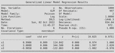
We can see that our fit is in good agreement with statsmodels, but we also get lots of other interesting information (coefficient uncertainty, NLL, deviance, etc.).

Correlations between two Poisson random variables

As mentioned in the introduction, if we have two Poisson random variables, $Z_1$ and $Z_2$, with no correlation (known as the ‘Double Poisson’ model) then the above approach still holds since the likelihood factorises:

$$\text{Po}(z_{1i},z_{2i}|{\lambda }_{1i},{\lambda }_{1i})=\frac{{\lambda }_{1i}^{z_{1i}}{e}^{-{\lambda }_{1i}}}{z_{1i}!}\cdot \frac{{\lambda }_{2i}^{z_{2i}}{e}^{-{\lambda }_{2i}}}{z_{2i}!}.$$

$$\begin{array}{rl}\Rightarrow \mathcal{L}({\lambda }_{1i},{\lambda }_{2i}|z_{1i},z_{2i})=\sum _i^n(& z_{1i}\log ({\lambda }_{1i})-{\lambda }_{1i}-\log (z_{1i}!))+\\ \sum _i^n(& z_{2i}\log ({\lambda }_{2i})-{\lambda }_{2i}-\log (z_{2i}!))\end{array}$$

and to maximise this we can just maximise the two sums separately. When doing so all of derivate crossterms, ${\partial }_{{\overrightarrow{\beta }}_n}{\overrightarrow{\lambda }}_m$, are zero for $n\ne m$ because of our ’no correlation’ rule.

But what if we suspect that our two random variables are correlated?

The Bivariate Poisson model deals with exactly this case – let $Y_0,Y_1,Y_2$ be independent univariate Poisson distributed with parameters ${\lambda }_1,{\lambda }_1,{\lambda }_2$ respectively. Then

$$\begin{array}{r}{Z}_0=Y_0+Y_2\\ Z_1=Y_1+Y_2\end{array}$$

are bivariate poisson distributed. Clearly $Z_0$ and $Z_1$ are maginally Poisson and therefore we have:

$$\begin{array}{r}\mathbb{E}[Z_0]={\lambda }_0+{\lambda }_2\\ \mathbb{E}[Z_1]={\lambda }_1+{\lambda }_2\end{array}$$

since sums of two independent Poisson distribution results in another Poisson parametrised by the sum of the two input distribution parameters. But more interestingly we also have

$$\begin{array}{rl}\text{Cov}(Z_0,Z_1)=& \text{Cov}(Y_0+Y_2,Y_1+Y_2)\\ =& \text{Cov}(Y_0,Y_1)+\text{Cov}(Y_0,Y_2)+\\ & \text{Cov}(Y_2,Y_1)+\text{Cov}(Y_2,Y_2)\\ =& \text{Cov}(Y_2,Y_2)\\ =& \text{Var}(Y_2)\\ =& {\lambda }_2.\end{array}$$

where $\text{Cov}(Y_i,Y_j)=0$ for $i\ne j$ by constrution of the $Y_j$’s.

The PMF of the Bivariate Poisson model is given by:

$$f_{\text{BP}}(Z_0,Z_1|{\lambda }_0,{\lambda }_1,{\lambda }_2)=e^{-{\lambda }_0-{\lambda }_1-{\lambda }_2}\frac{{\lambda }_0^{z_0}}{z_0!}\frac{{\lambda }_1^{z_1}}{z_1!}\sum _{k=0}^{min(z_0,z_1)}(\genfrac{}{}{0ex}{}{z_0}{k})(\genfrac{}{}{0ex}{}{z_1}{k})k!{\left(\frac{{\lambda }_2}{{\lambda }_1{\lambda }_1}\right)}^k$$

We can see that when ${\lambda }_2\to 0$ this reduces to the Double Poisson model since only the $k=0$ term in the sum contributes and it contributes $1$, leaving only the coefficient in front remaining.

The problem we now have to solve then is:

$$\begin{array}{rl}{Z}_{0i},Z_{1i}& \sim \text{BP}(Z_{0i},Z_{1i}|{\lambda }_{0i},{\lambda }_{1i},{\lambda }_{2i})\\ \log {\lambda }_{ki}& =\overrightarrow{{\beta }_k}\cdot \overrightarrow{x_i}\end{array}$$

where $i$ indexes over the paired datapoints and $k=1\dots 3$, and associated covariates. It is possible that the ${\lambda }_k$ depend on different (or even distinct) subsets of the covariates, but we can always treat this case using a single $\overrightarrow{x_i}$ created by concatenating the different features and enforcing that the pertinent components of $\beta$ are zero.

Fitting the Bivariate Poisson with the EM algorithm

We saw above that we can directly maximise the likelihood of a univariate Poisson distribution, but with the Bivariate Poisson case it is more awkward. Here I’m going to follow the approach taken in the Karlis and Ntzoufras paper ² and take an Expectation-Maximisation approach ^{3 4}. I also recommend Ntzoufras’s book which describes lots of interested models ⁵.

Computing The Likelihood

We can write down a seemingly useless for for the bivariate model, one expressed in terms of all three of the unobserved Poisson components:

$$f(Y_0,Y_1,Y_2|\mathrm{\Theta })=\prod _{i=1}^n\prod _{k=1}^3\frac{e^{-{\lambda }_i}{\lambda }_i^{y_k}}{y_k!}$$

We can perform a change of variables so that our model is in terms of the two observed random variables $(Z_0,Z_1)$ and a single latent variable $Y_2$, the determinant of the Jacobian of the transformation is 1 so we have

$$\begin{array}{r}L({\lambda }_0,{\lambda }_1,{\lambda }_2|Z_0,Z_1,Y_2)=\prod _{i=1}^n\frac{e^{-{\lambda }_0}{\lambda }_0^{z_{0i}-y_{2i}}}{(z_{0i}-y_{2i})!}\frac{e^{-{\lambda }_1}{\lambda }_1^{z_{1i}-y_{2i}}}{(z_{1i}-y_{2i})!}\frac{e^{-{\lambda }_2}{\lambda }_2^{y_{2i}}}{y_{2i}!}\end{array}$$

and therefore the log-likelihood is

$$\begin{array}{rl}\mathcal{L}({\lambda }_0,{\lambda }_1,{\lambda }_2|Z_0,Z_1,Y_2)=-& n{\lambda }_0+\sum _{i=1}^n(z_{0i}-y_{2i})\log {\lambda }_0-\log \prod _{i=1}^n(z_{0i}-y_{2i})!\\ -& n{\lambda }_1+\sum _{i=1}^n(z_{1i}-y_{2i})\log {\lambda }_1-\log \prod _{i=1}^n(z_{1i}-y_{2i})!\\ -& n{\lambda }_2+\sum _{i=1}^n{y}_{2i}\log {\lambda }_2-\log \prod _{i=1}^n{y}_{2i}!\end{array}$$

This is almost the same as the ‘Double Poisson’ model and we know we can maximise it with respect to the $\lambda$’s, except that we don’t know the value of the $y_{2i}$. This is where the Expectation-Maximisation algorithm comes in.

Computing The Density of the Latent Variable

To get the $\mathcal{Q}$ function we need to compute the expectation of the log-likelihood with respect to the density $f(Y_2|Z_0,Z_1,{\lambda }_k^{(t)})$, where ${\lambda }_k^{(t)}$ are our current guess for the lambdas. Using Baye’s theorem we can write this as:

$$f(Y_2|Z_0,Z_1,{\lambda }_k^{(t)})=\frac{f(Z_0,Z_1|Y_2,{\lambda }_k^{(t)})f(Y_2|{\lambda }_k^{(t)})}{f(Z_0,Z_1|{\lambda }_k^{(t)})}$$

The denominator is just the Bivariate Poisson density and $f(Y_2|{\lambda }_k^{(t)})$ is just the Poisson density. The last term, $f(Z_0,Z_1|Y_2,{\lambda }_k^{(t)})$, is a little harder to reason about – but if we look to the definitions $Z_0,Z_1$ and imagine that $Y_2$ is just a constant we see the following is true

$$f(Z_0,Z_1|Y_2,{\lambda }_k^{(t)})=f(Y_0=Z_0-Y_2|{\lambda }_k^{(t)})f(Y_1=Z_1-Y_2|{\lambda }_k^{(t)})$$

and both of the distributions on the right-hand side are just more Poisson distributions. Thus:

$$f(Y_2|Z_0,Z_1,{\lambda }_k^{(t)})=\frac{\text{Po}(Y_0=Z_0-Y_2|{\lambda }_k^{(t)})\text{Po}(Y_1=Z_1-Y_2|{\lambda }_k^{(t)})\text{Po}(Y_2|{\lambda }_k^{(t)})}{f_{\text{BP}}(Z_0,Z_1|{\lambda }_k^{(t)})}$$

Computing The Expectation of the Latent Variable

With this density computed we can compute the expectation of the unobserved $Y_2$ conditioned on the observed data:

$${\mathbb{E}}_{Y_2|Z_0,Z_1,{\lambda }_k^{(t)}}[Y_2]=\sum _{j=0}^{\mathrm{\infty }}j\frac{\text{Po}(z_0-j|{\lambda }_0)\text{Po}(z_1-j|{\lambda }_1)\text{Po}(j|{\lambda }_2)}{f_{\text{BP}}(Z_0,Z_1|{\lambda }_k^{(t)})}$$

The denominator is independent of our index, $j$, and we can change the bounds of the summation in two ways:

• Firstly we can use that fact that the $j=0$ term in the sum is clearly zero to shift the start of the summation,
• Secondly we see that for any $j>z_0$ or $j>z_1$ the Poisson density is zero (the domain of the Poisson is non-negative integers). Therefore the upper bound of the sum is $max(z_0,z_1)$.

Therefore

$$\mathbb{E}[Z_0]=\frac{1}{f_{\text{BP}}(Z_0,Z_1|{\lambda }_k^{(t)})}\sum _{j=1}^{max(z_0,z_1)}j\text{Po}(z_0-j|{\lambda }_0)\text{Po}(z_1-j|{\lambda }_1)\text{Po}(j|{\lambda }_2)$$

Substituting in the density of the Poisson (and suppressing, for now, the EM iteration index $(t)$)

$$\mathbb{E}[Z_0]=\frac{1}{f_{\text{BP}}(Z_0,Z_1|{\lambda }_k)}\sum _{j=1}^{max(z_0,z_1)}j\frac{{\lambda }_0^{z_0-j}{e}^{{\lambda }_0}}{(z_0-j)!}\frac{{\lambda }_1^{z_1-j}{e}^{{\lambda }_1}}{(z_1-j)!}\frac{{\lambda }_2^j{e}^{{\lambda }_2}}{j!}$$

We can pull out some factors of the lambdas:

$$\mathbb{E}[Z_0]=\frac{{\lambda }_2{e}^{-{\lambda }_0-{\lambda }_1-{\lambda }_2}{\lambda }_0^{z_0-1}{\lambda }_1^{z_1-1}}{f_{\text{BP}}(Z_0,Z_1|{\lambda }_k)}\sum _{j=1}^{max(z_0,z_1)}j\frac{1}{(z_0-j)!(z_1-j)!j!}{\left(\frac{{\lambda }_2}{{\lambda }_1{\lambda }_1}\right)}^{j-1}$$

Now some more index trickery, we let $p=j-1$ in the sum:

$$\begin{array}{rl}=& \frac{{\lambda }_2{e}^{-{\lambda }_0-{\lambda }_1-{\lambda }_2}{\lambda }_0^{z_0-1}{\lambda }_1^{z_1-1}}{f_{\text{BP}}(Z_0,Z_1|{\lambda }_k)}\dots \\ & \sum _{p=0}^{max(z_0-1,z_1-1)}(p+1)\frac{1}{(z_0-p-1)!(z_1-p-1)!(p+1)!}{\left(\frac{{\lambda }_2}{{\lambda }_1{\lambda }_1}\right)}^p\\ =& \frac{{\lambda }_2{e}^{-{\lambda }_0-{\lambda }_1-{\lambda }_2}{\lambda }_0^{z_0-1}{\lambda }_1^{z_1-1}}{f_{\text{BP}}(Z_0,Z_1|{\lambda }_k)(z_0-1)!(z_1-1)!}\dots \\ & \sum _{p=0}^{max(z_0-1,z_1-1)}\frac{(z_0-1)!(z_1-1)!}{(z_0-p-1)!(z_1-p-1)!p!}{\left(\frac{{\lambda }_2}{{\lambda }_1{\lambda }_1}\right)}^p\end{array}$$

we recognise the combination of factorials inside the sum as binomial coefficients

$$\begin{array}{rl}=& \frac{{\lambda }_2{e}^{-{\lambda }_0-{\lambda }_1-{\lambda }_2}{\lambda }_0^{z_0-1}{\lambda }_1^{z_1-1}}{f_{\text{BP}}(Z_0,Z_1|{\lambda }_k)(z_0-1)!(z_1-1)!}\sum _{p=0}^{max(z_0-1,z_1-1)}(\genfrac{}{}{0ex}{}{z_0-1}{p})(\genfrac{}{}{0ex}{}{z_1-1}{p})p!{\left(\frac{{\lambda }_2}{{\lambda }_1{\lambda }_1}\right)}^p\end{array}$$

and finally we have:

$$\begin{array}{r}{y}_2^{(t)}\equiv {\mathbb{E}}_{Y_2|Z_0,Z_1,{\lambda }_k^{(t)}}[Y_2]={\lambda }_2\frac{f_{\text{BP}}(Z_0-1,Z_1-1|{\lambda }_k^{(t)})}{f_{\text{BP}}(Z_0,Z_1|{\lambda }_k^{(t)})}\end{array}$$

The EM algorithm

The auxilliary function, $\mathcal{Q}$, is then just the log-likelihood where we use the expected value for the latent variable we just computed

$$\begin{array}{rl}\mathcal{Q}(\lambda |{\lambda }_k^{(t)})=-& n{\lambda }_0+\sum _{i=1}^n(z_{0i}-y_{2i}^{(t)})\log {\lambda }_0\\ -& n{\lambda }_1+\sum _{i=1}^n(z_{1i}-y_{2i}^{(t)})\log {\lambda }_1\\ -& n{\lambda }_2+\sum _{i=1}^n{y}_{2i}^{(t)}\log {\lambda }_2.\end{array}$$

where the terms which don’t depend on ${\lambda }_k$ have been dropped. Remembering for a moment that the lambdas are themselves functions of the regression weights:

$$\log {\lambda }_{ki}=\overrightarrow{{\beta }_k}\cdot \overrightarrow{x_i}$$

we can see that to maximise the $\mathcal{Q}$ function we have to perform three separate Poisson regressions:

to compute the weights $\beta$. In summary then the EM iterations look like this:

• E-step: Using our current best guess for the model weights, ${\beta }^{(t-1)}$, we compute $y_{2i}^{(t)}$ for each datapoint,
• M-step: We perform the follow three Poisson regressions $$\begin{array}{rl}{z}_{0i}-y_{2i}^{(t)}& \sim \text{Po}({\lambda }_{0i}^{(t-1)}),\log {\lambda }_{0i}^{(t-1)}={\overrightarrow{{\beta }_0}}^{(t-1)}\cdot \overrightarrow{x_i}\\ z_{1i}-y_{2i}^{(t)}& \sim \text{Po}({\lambda }_{1i}^{(t-1)}),\log {\lambda }_{1i}^{(t-1)}={\overrightarrow{{\beta }_1}}^{(t-1)}\cdot \overrightarrow{x_i}\\ y_{2i}^{(t)}& \sim \text{Po}({\lambda }_{2i}^{(t-1)}),\log {\lambda }_{2i}^{(t-1)}={\overrightarrow{{\beta }_2}}^{(t-1)}\cdot \overrightarrow{x_i}\end{array}$$

to find our next estimates for the model weights ${\overrightarrow{{\beta }_2}}^{(t)}$.

Implementation in python

And now lets implement all of this in python. We start by generating the latent $Y_j$ data from independent Poissons and the combining them to form the $Z_i$:

@dataclass
class LatentData:
    lambdas: np.array
    Y0: np.array
    Y1: np.array
    Y2: np.array

@dataclass
class BivariateData:
    dims: Dims
    latent: LatentData
    observed: ObservedData

def generate_observed_bivariate_poisson_data(YY_latent: np.array) -> np.array:
    return np.stack([
        YY_latent[0,:] + YY_latent[2,:],
        YY_latent[1,:] + YY_latent[2,:],
    ])

def generate_bivariate_poisson_data(true_betas: np.array, N: int, sigma: float) -> BivariateData:
    M = true_betas.shape[0]
    covariates = np.random.normal(0, sigma, (N, M))
    # Fix the first row to allow for a constant term in the regression
    covariates[0, :] = 1
    # Build the lambdas from the betas, and then sample from the Poissons
    lambdas = np.exp(covariates.dot(true_betas))
    latent_poisson_draws = np.random.poisson(lambdas)
    observations = generate_observed_bivariate_poisson_data(latent_poisson_draws.T)
    return BivariateData(
        Dims(N, M),
        LatentData(lambdas, *latent_poisson_draws.T),
        ObservedData(covariates, *observations),
    )

true_betas = np.array([
    [0.3,  0.2,  0.0,  0.3, 0.0,  0.0],
    [0.5,  0.0, -0.1,  0.0, 0.0, -0.5],
    [0.0,  0.0,  0.0,  0.0, 1.0,  0.0],
]).T

dataset = generate_bivariate_poisson_data(true_betas, N=10000, sigma=1)

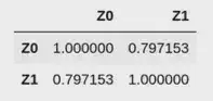
We can check the correlation matrix of the latent data, and the observed data to see that this has worked as expected:

import pandas as pd

pd.DataFrame(
    data=np.array([
        dataset.latent.Y0,
        dataset.latent.Y1,
        dataset.latent.Y2,
    ]).T,
    columns=['Y0', 'Y1', 'Y2']
).corr()

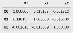
import pandas as pd

pd.DataFrame(
    data=np.array([
        dataset.observed.Z0,
        dataset.observed.Z1,
    ]).T,
    columns=['X0', 'X1']
).corr()

The $Z_i$’ have a strong degree of correlation, so far so good. We need the Bivariate Poisson density, $f_{\text{BP}}(Z_0,Z_1|{\lambda }_0,{\lambda }_1,{\lambda }_2)$:

from scipy.special import factorial

EPS = 1e-16

def choose(n: int, p: int) -> int:
    return factorial(n) / factorial(p) / factorial(n - p)

def bivariate_poisson(x: int, y: int, l0: float, l1: float, l2: float) -> float:
    coeff = (
        np.exp(-l0 - l1 - l2) * np.power(l0, x) *
        np.power(l1, y) / factorial(x) / factorial(y)
    )
    p = coeff * sum([
        choose(x, i) * choose(y, i) * factorial(i) * (l2 / l0 / l1) ** i
        for i in range(0, min(x, y) + 1)
    ])
    return max(p, EPS)

For the E-step of the EM algorithm we must compute the expectation $y_2^{(t)}={\mathbb{E}}_{Y_2|Z_0,Z_1,{\lambda }_k^{(t)}}[Y_2]$ for each datapoint, $i$:

def _compute_next_y2ti(x, y, l0, l1, l2):
    if min(x, y) < 1:
        return 0
    return l2 * bivariate_poisson(x - 1, y - 1, l0, l1, l2) / bivariate_poisson(x, y, l0, l1, l2)

def compute_next_y2ti(observed_data: ObservedData, lambdas: np.array) -> np.array:
    return np.array([
        _compute_next_y2ti(z0, z1, *lams)
        for (z0, z1, lams) in zip(observed_data.Z0, observed_data.Z1, lambdas)
    ])

For the M-step we can re-use the 1D Poisson regression code from earlier in this post to compute the betas, and from the betas we get our new estimate for the lambdas:

def compute_next_betas(
    data: BivariateData,
    y2ti: np.array,
) -> np.array:
    return np.array([
        poisson_regression(data.observed.covariates, data.observed.Z0 - y2ti),
        poisson_regression(data.observed.covariates, data.observed.Z1 - y2ti),
        poisson_regression(data.observed.covariates, y2ti),
    ]).T

def compute_next_lambdas(betas, covariate_matrix):
    return np.exp(covariate_matrix.dot(betas))

That is everything we really need to fit this model, but to make the output more interesting we should include a little extra code to track the negative log-likelihood of the model, and the mean squared error to see that the EM algorithm is converging:

@dataclass
class FitResult:
    betas: np.array
    neg_loglikelihood: float

def bivariate_poisson_nll(betas: np.array, observed_data: ObservedData):
    lambdas = np.exp(observed_data.covariates.dot(betas))
    return -np.sum([
        np.log(bivariate_poisson(z0, z1, *lams))
        for (z0, z1, lams) in zip(observed_data.Z0, observed_data.Z1, lambdas)
    ])

def bivariate_poisson_prediction(betas, observed_data: ObservedData):
    lambdas = np.exp(observed_data.covariates.dot(betas))
    return np.stack([lambdas[:, 0] + lambdas[:, 2], lambdas[:, 1] + lambdas[:, 2]])

def compute_mse(predictions, Z0, Z1):
    return np.mean((predictions[0,:] - Z0 + predictions[1,:] - Z1) ** 2)

def compute_bivariate_poisson_data_mse(betas: np.array, observed_data: ObservedData) -> float:
    preds = bivariate_poisson_prediction(betas, observed_data)
    return compute_mse(preds, observed_data.Z0, observed_data.Z1)

And finally we fit the model:

def bivariate_poisson_fit_using_em(
    dataset: BivariateData,
    em_max_itr: int=20,
    logging: bool=False
) -> FitResult:
    # Construct some initial guesses for the lambdas and betas
    betas = np.zeros((dataset.dims.M, 3))
    lambdas = compute_next_lambdas(betas, dataset.observed.covariates)

    for itr in range(1, em_max_itr + 1):
        nll = bivariate_poisson_nll(betas, dataset.observed)
        bivpoisson_mse = compute_bivariate_poisson_data_mse(betas, dataset.observed)
        if logging:
            print(f"{itr:<4} {nll:<10.3f} {bivpoisson_mse:.3f}")

        # E-step:
        y2ti = compute_next_y2ti(dataset.observed, lambdas)

        # M-step:
        betas = compute_next_betas(dataset, y2ti)
        lambdas = compute_next_lambdas(betas, dataset.observed.covariates)

    return FitResult(betas, nll)

fit_bp = bivariate_poisson_fit_using_em(dataset, provide_model_structure=False, logging=True)

>>> 1    45134.088  33.348
>>> 2    34808.743  11.267
>>> 3    34207.242  10.415
>>> 4    33747.553  9.645
>>> 5    33498.612  9.208
>>> 6    33406.624  9.064
>>> 7    33381.469  9.042
>>> 8    33375.651  9.046
>>> 9    33374.371  9.052
>>> 10   33374.077  9.054

we can compare the model fitted $\beta$ values to the true $\beta$’s and see that they are in good agreement:

fit_bp.betas.round(2).T
>>> array([[ 0.3 ,  0.21, -0.  ,  0.3 ,  0.  ,  0.02],
>>>        [ 0.5 , -0.  , -0.1 , -0.01, -0.01, -0.5 ],
>>>        [-0.  , -0.01, -0.01, -0.01,  1.  ,  0.  ]])

true_betas.round(2).T
>>> array([[ 0.3,  0.2,  0. ,  0.3,  0. ,  0. ],
>>>        [ 0.5,  0. , -0.1,  0. ,  0. , -0.5],
>>>        [ 0. ,  0. ,  0. ,  0. ,  1. ,  0. ]])

We can also perform a Double Poisson fit and compare the MSE of the two models.

def double_poisson_fit(data: BivariateData) -> FitResult:
    betas = np.array([
        poisson_regression(data.observed.covariates, data.observed.XX),
        poisson_regression(data.observed.covariates, data.observed.YY),
    ]).T
    return FitResult(betas)

def double_poisson_prediction(betas, data: ObservedData):
    lambdas = np.exp(data.covariates.dot(betas))
    return np.stack([lambdas[:, 0], lambdas[:, 1]])

fit_dp = double_poisson_fit(dataset)
preds_dp = double_poisson_prediction(fit_dp.betas, dataset.observed)
print(compute_mse(preds_dp, dataset.observed.XX, dataset.observed.YY))
>>> 16.204314367381187

which is significantly worse than the 9.054 managed by the Bivariate Poisson regression.

References